Software Design
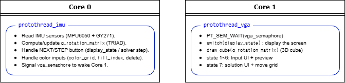
The program is split across two RP2040 cores: Core0 acquires sensors and user input and updates the rotation matrix, while Core1 focuses on VGA rendering and UI drawing. Core0 signals Core1 via a semaphore to refresh the display using the latest orientation estimate and UI state.
Overall Architecture
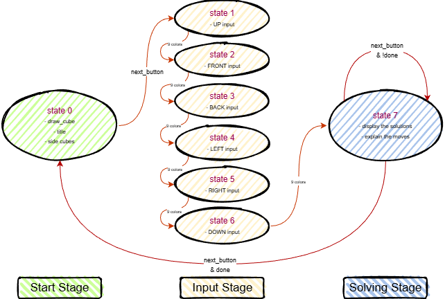
The overall software architecture is summarized below. The state machine organizes the user workflow from live 3D viewing, through face-by-face color entry, to step-by-step solution playback.
Orientation Estimation (TRIAD)
We used TRIAD to estimate cube orientation in real time and drive the live 3D Rubik’s Cube visualization on VGA. At each update, the accelerometer vector is used as \(\mathbf{v}_1\), and the magnetometer vector is used as \(\mathbf{v}_2\).
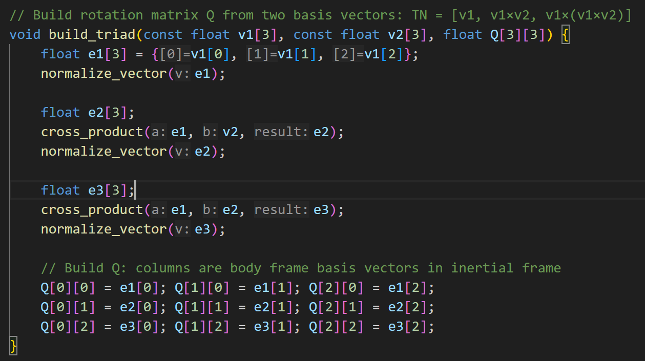
From these two non-collinear vectors, we construct an orthonormal basis: \(\mathbf{e}_1=\hat{\mathbf{v}}_1\), \(\mathbf{e}_2=\widehat{\mathbf{e}_1\times \mathbf{v}_2}\), and \(\mathbf{e}_3=\mathbf{e}_1\times\mathbf{e}_2\), so that \(\mathbf{T}=[\mathbf{e}_1\ \mathbf{e}_2\ \mathbf{e}_3]\).
Since \(\mathbf{T}_N\) and \(\mathbf{T}_B\) are orthonormal, \(\mathbf{T}^{-1}=\mathbf{T}^T\), and: \[ \mathbf{Q}=\mathbf{T}_B\mathbf{T}_N^{T}. \]
Expanded TRIAD form (as referenced in the report):
\[ {}^{N}\!Q^{B} = {}^{N}\!\left[ \hat{\mathbf v}_1 \;\; (\hat{\mathbf v}_1 \times \hat{\mathbf v}_2) \;\; \bigl(\hat{\mathbf v}_1 \times (\hat{\mathbf v}_1 \times \hat{\mathbf v}_2)\bigr) \right]\, \left( {}^{B}\!\left[ \hat{\mathbf v}_1 \;\; (\hat{\mathbf v}_1 \times \hat{\mathbf v}_2) \;\; \bigl(\hat{\mathbf v}_1 \times (\hat{\mathbf v}_1 \times \hat{\mathbf v}_2)\bigr) \right] \right)^{-1}. \]
Real-Time 3D Cube Rendering
We rotate the cube’s eight predefined 3D vertices using \(\mathbf{Q}^T\) and map the rotated coordinates onto the VGA display using an orthographic projection with a fixed scale factor.
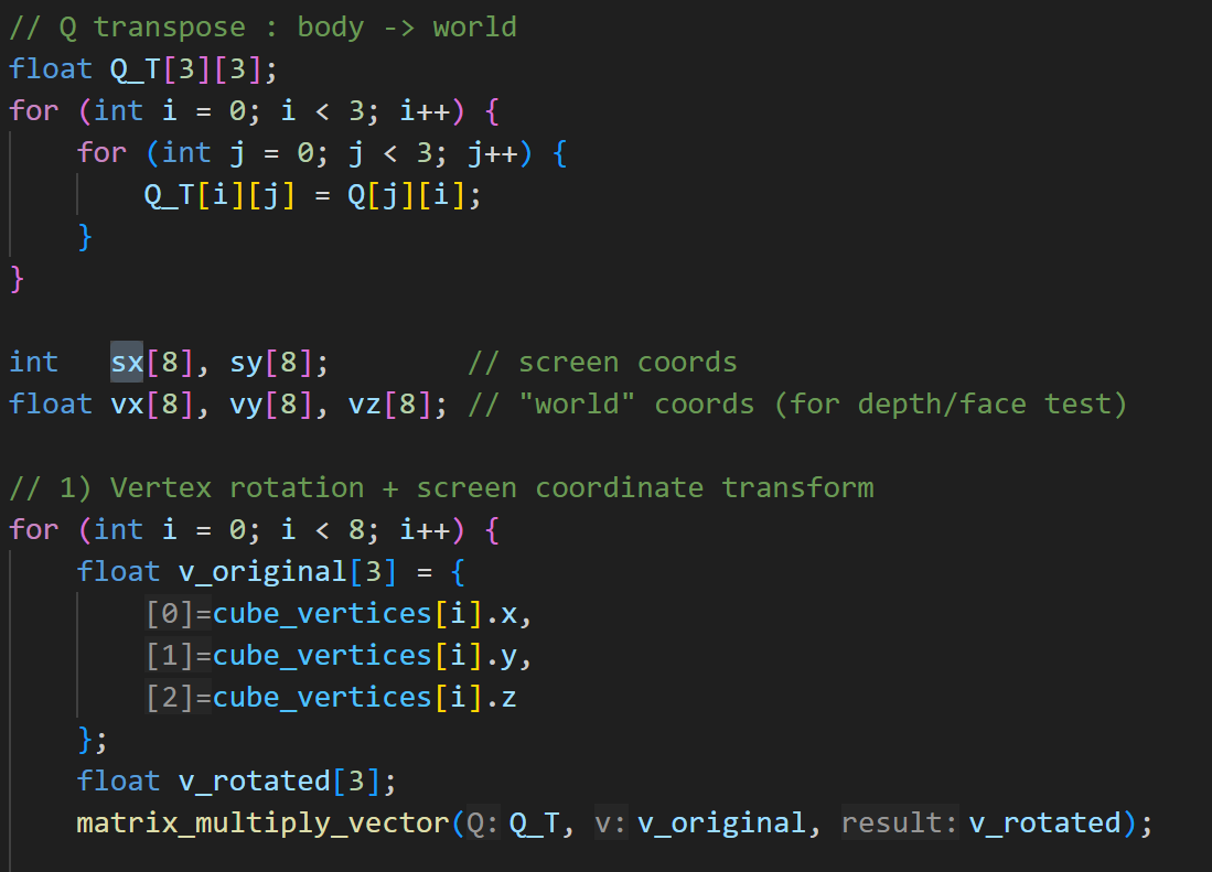
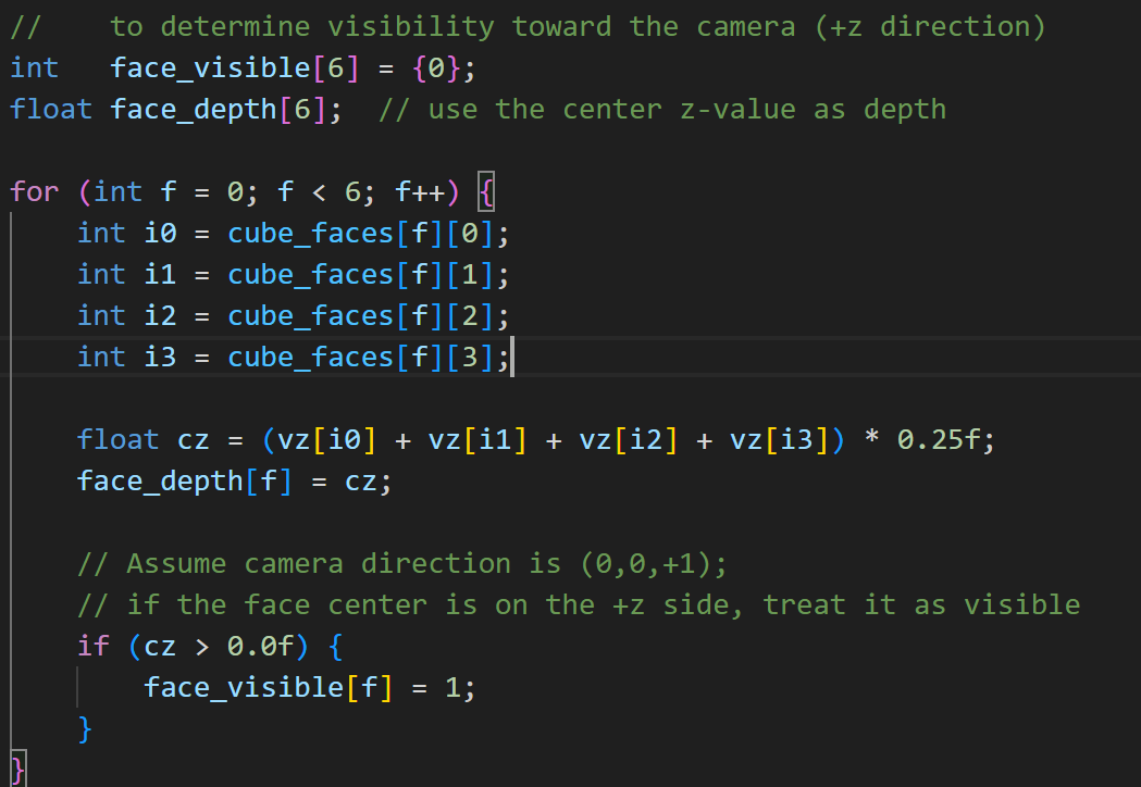
To render solid faces, we estimate each face’s depth using the average \(z\) value of its vertices, treat faces with positive depth as visible, and draw them from far to near. Each visible face is divided into a \(3\times3\) grid and filled using triangles, with grid lines overlaid to complete the 3D Rubik’s Cube visualization.
Consistent Face Mapping
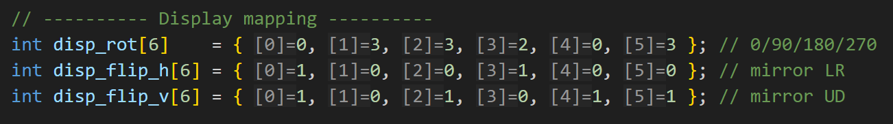
We adopted a fixed solver convention for the six faces and stored the cube state in a \(6\times3\times3\) sticker array. Each entered face grid is converted into this canonical representation via a face-specific in-plane rotation and (if needed) mirroring, ensuring consistent mapping between UI input, internal model, and rendering.
Solving Algorithm and Execution (IDDFS)
After the user finishes entering all six faces, we convert the six \(3\times3\) color grids into the internal cube state. We then search for a solution using iterative deepening depth-first search (IDDFS) with a limited move set.
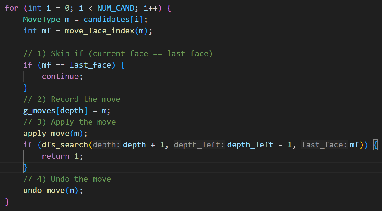
At each depth, DFS enumerates candidate moves and performs backtracking: record the current move, apply it, recursively search, and undo it if the recursive call fails. Once a valid sequence is found, we restore the cube to the original state, save the move list, and allow the user to apply one move per NEXT press in solver mode.
User Interface State Machine
The UI is organized into three stages: State 0 (live IMU-tracked 3D cube), States 1–6 (face-by-face color entry), and State 7 (solution display and step-by-step application). NEXT advances states and applies moves in State 7.