 Introduction
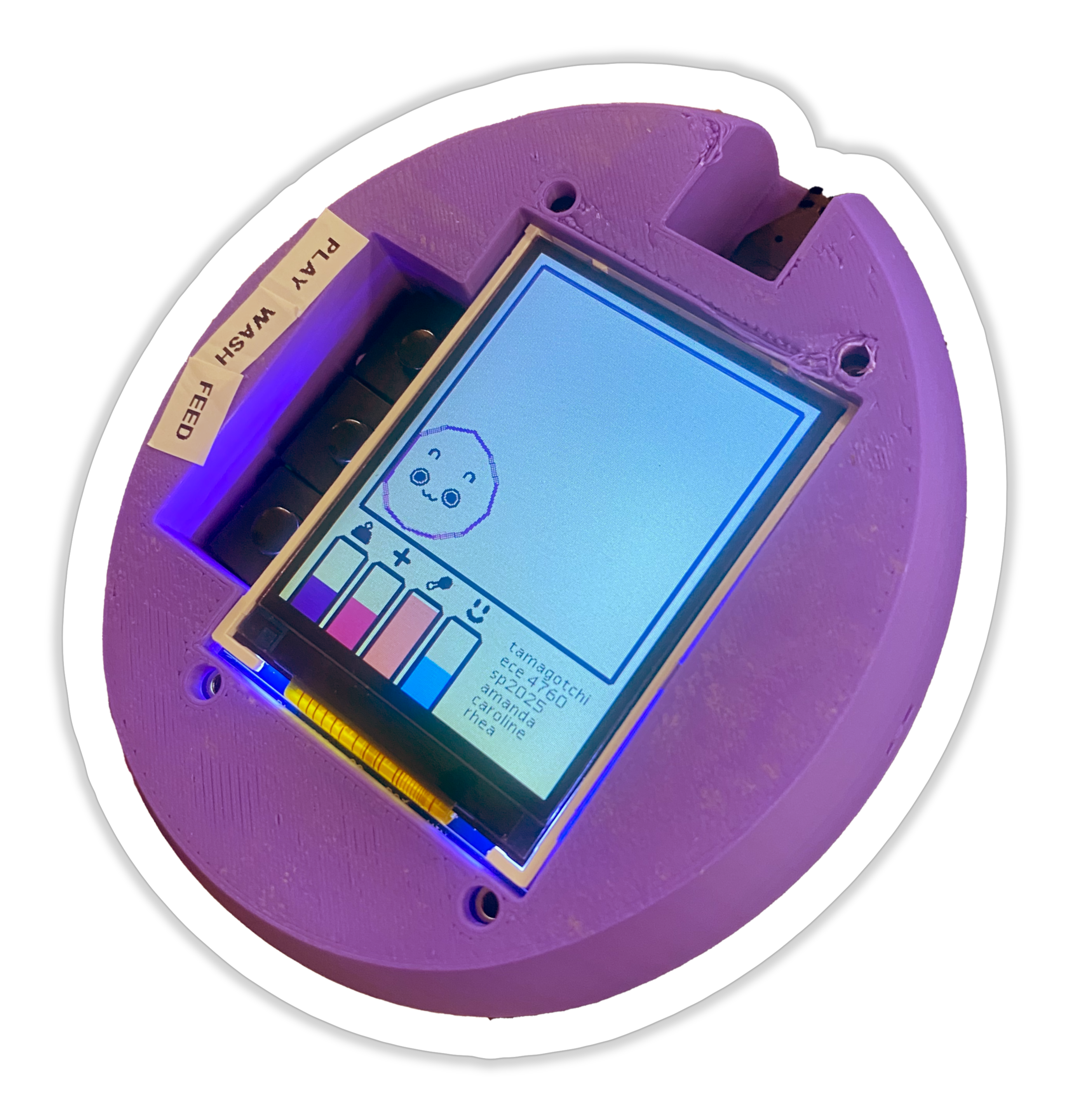
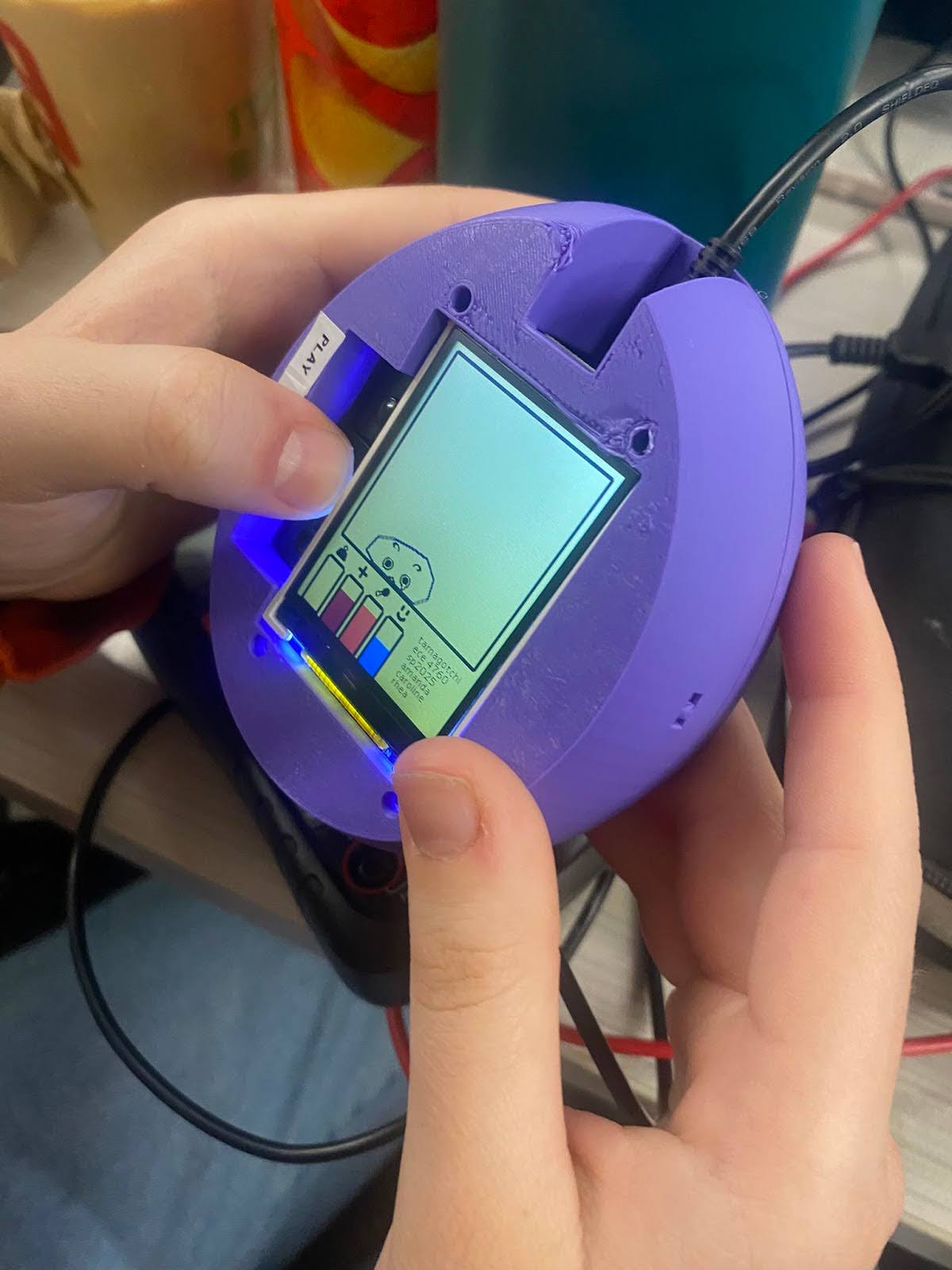
Do not be alarmed by the name of our project! Ok, maybe be a little alarmed. The Tamagotchi Torture Chamber combines the iconic 90s toy with a soft-body physics simulation and an accelerometer, allowing users to roll a squishy pet around a digital enclosure. The Tamagotchi Torture Chamber is a fully hand-held device that persists the state of your pet across boots, so they can never forget what you've done to them. Our soft-body physics simulation is based on the 2004 paper "How to implement a pressure soft body model" by Maciej Matyk. The creature is represented by a ring of vertices, with adjacent vertices connected by springs. Internal pressure, responsible for maintaining the creature's roughly spherical shape, is derived from its current surface area. Put together, we have a shape that can collapse on collisions but generally maintain its shape.
When you first power on a new Tamagotchi Torture Chamber, a default initial state is persisted in external memory (FRAM). However, on subsequent boots, your pet’s previous state is automatically loaded so you can pick up right where you left off!
Using the three buttons located on the side of the TTC, you can interact with your pet! Feed it, play with it, or clean it. Your pet has four stats: weight, food, happiness, and health. Feeding your pet increases its food meter as well as its weight. Playing with your pet increases its happiness meter and decreases its weight. Cleaning your pet increases its health, but decreases its happiness. If you let any of these stats get too low (or too high, for weight), your pet will start crying. If all of these stats fall to 0, or you overfeed your pet, it will die. Not to worry, though, because pressing any button after your pet dies will reset it.
Of course, you may also interact with the pet by knocking it around its enclosure. If your pet slams against any wall too hard, it will look dizzy and its health will decrease. Tilt the TTC to slide your pet around and watch it squish up against the walls.
High-Level Design
Rationale
Our project was motivated by our desire to create a silly little game that was portable and a little twisted. It was also motivated by Caroline’s interest in game design and video games and our desire to put a technical swing on a more visual project. By adding extra devices like the FRAM and IMU, we turned our game into a comprehensive electrical system design project. We wanted to develop an interactive game that a lot of people have experience with. We also wanted to have a game that the user could “take on the go” with them, and we felt like adding acceleration to change the little digital pet’s motion was the perfect touch of user interaction. We honestly thought the Tamagotchi was adorable and wanted to put our twist on the game. Our project draws inspiration from digital display (not the VGA, however) from Lab 2: Digital Galton Board and calculating IMU orientation in Lab 3: PID control of a 1D helicopter.
Background Math: Softbody Physics Simulation
We simulate softbody physics in our game play as a user interaction with your pet as a result of the IMU readings. Unlike rigid bodies, the shape of soft bodies can change as they have force applied to them (either from other bodies or their environment like colliding with a wall). We can decompose a soft body to be an n-polygon where n is the number of vertices on the polygon. Each vertex of the polygon is connected to a spring which connects to an adjacent vertex, which can be seen in the figure below.
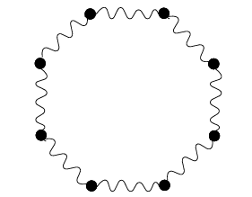 Fig. 1: Adjacent vertices are connected by springs, creating the
impression of a soft body. Image from Maciej Matyka’s paper.
Fig. 1: Adjacent vertices are connected by springs, creating the
impression of a soft body. Image from Maciej Matyka’s paper.
The forces acting on each vertex are summed (both external from gravity and internal from the springs). There is also an internal pressure force that dictates how much the soft body deflates when the force is applied, but it is a constant that requires tuning to make sure that the soft body does not completely lose its shape when it deflates. Then, Euler Integration is applied to find the next position of each vertex.
Since we do not have another body in our simulation, the only collisions we have to detect are those against the wall. We are able to detect those collisions through checks in the physics thread, which checks if any of the vertices on the soft body was outside the TFT screen dimensions. If this was the case, then we inverted the velocity in that direction to create a “bounce” effect for the soft body.
Logical Structure
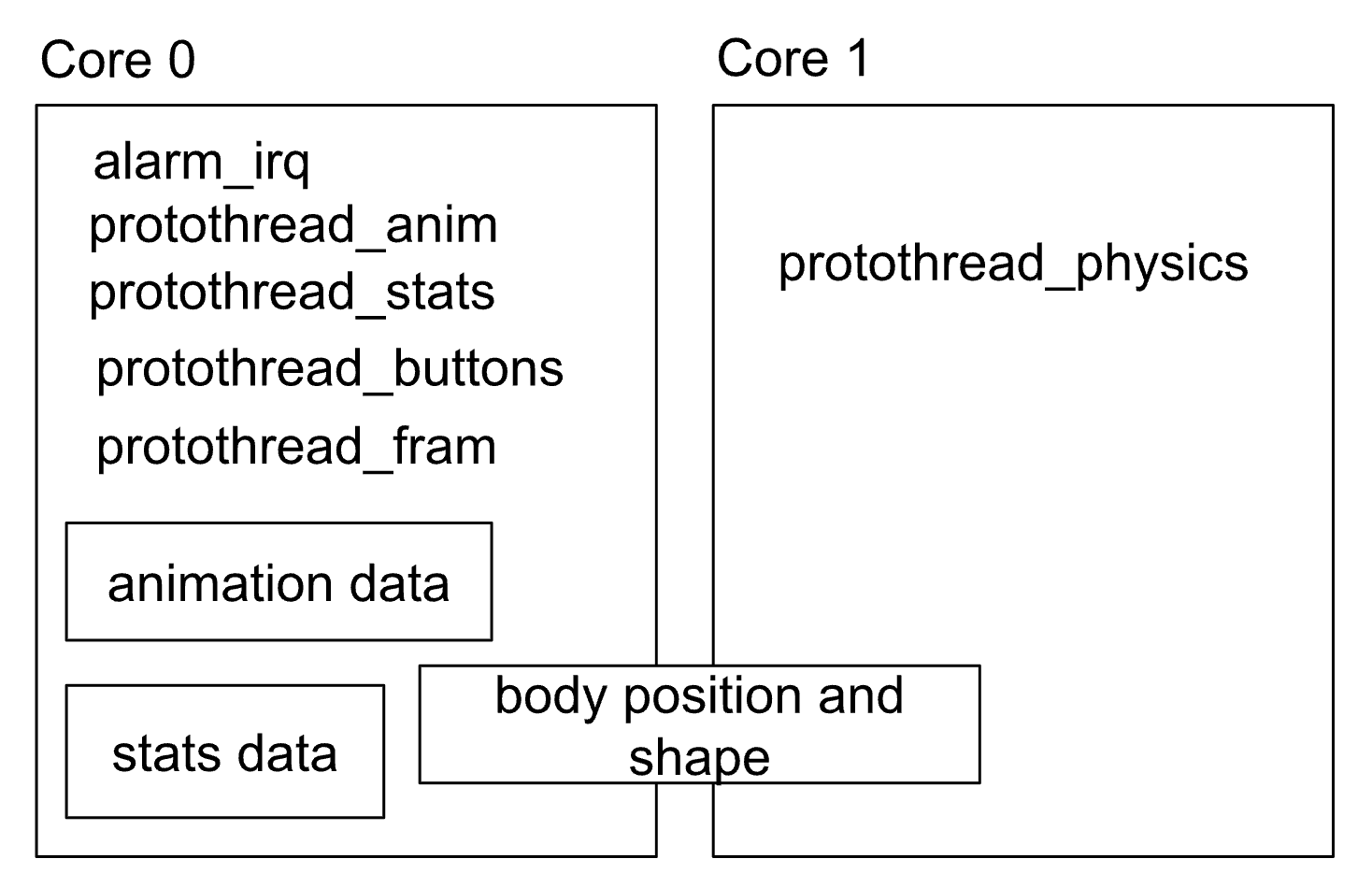 Fig. 2: General layout of the TTC's code, excluding driver
implementations. The three smaller boxes represent shared state data,
positioned by users.
Fig. 2: General layout of the TTC's code, excluding driver
implementations. The three smaller boxes represent shared state data,
positioned by users.
Our code is divided into five threads and an alarm IRQ, with the physics simulation thread running on core 1 (and the rest on core 0). We have threads for UI updates, drawing the sprite canvas, running the physics simulation, updating the FRAM device, and polling button input from users. These threads share data regarding the screen-space location of each vertex in the soft body and the stats of the pet. The IRQ is responsible for polling acceleration data from the IMU.
Hardware/Software Tradeoffs
The hardware tradeoffs that we decided on were between using the full RP2040 that we were provided from previous labs or a mini RP2040. Ultimately, we decided to use the full RP2040 because the VGA screen fully covered the RP2040. We also decided that the full RP2040 made it easier for us to solder connections to the solder perfboard. However, it did make our Tamagotchi egg thicker than expected. Another hardware tradeoff that we had was soldering all of our connections to keep them robust and sturdy while we play the game. To limit the clunkiness of the egg case, we decided to not make our tamagotchi fully portable. This is because the battery holder for 2 AA batteries to power full RP2040 was a couple inches thick. For the software tradeoffs, we decided to put everything but the physics logic on core 0. The physics logic was put on core 1 because it was the only computationally heavy thread and we needed the physics logic to be fast. So, the physics protothread needed all the CPU to be allocated to it. Another software tradeoff that we had was the level of detail with animations compared to the efficiency of the drawing calls.
Relevant Work
Our project is based on the product, Tamagotchi, which has a US Patent from 1997. Thus, our primary intellectual property consideration is the function and the design of the game itself. The patent describes several things unique to the Tamagotchi game, which are its icons for interactions (surrounding the little pet), the drawing of the little pet itself, the egg structure, and the logic behind how the user can interact with this game. Though we are drawing lots of inspiration from the original Tamagotchi functionality and essence, we fully intend to make it our own by having our own interactions and procedure for how to keep the Tamagotchi alive (which will be more simplistic than the original Tamagotchi game) and our little digital pet will be one of our own design. We aim to emulate the things that made the Tamagotchi unique, such as its egg shape and the interactions with the digital pet, to invoke that sense of familiarity and nostalgia with our users to increase usability of our game. However, that is where our similarities will stop as we will create the rest based on our own ideas and add new features (such as movement of the pet around the screen).
As we previously mentioned, our physics simulation is based on the 2004 paper "How to implement a pressure soft body model" by Maciej Matyk. This is a pretty common model for implementing soft-body physics, with one of the main points of deviation being the layout of the springs.
Safety
Mostly because our device comes in a printed case which prevents user access to the hardware, we do not see any safety or hardware concerns.
Programming & Hardware Design
Graphics
We adapted Parth Sharma's driver for the TFT screen to optimize and improve our graphics. Instead of the full 16-bit color spectrum allowed by the driver, we are using an indexed color scheme based on the Sweetie 16 palette by GrafxKid on Lospec. This allows us to maintain a consistent aesthetic and pack our images into smaller bitmaps, needing only one byte per pixel.
 Fig. 3: One of GrafxKid's examples of their Sweetie 16 palette.
Images in our project are stored in flash memory as byte arrays, where every byte contains the index of a pixel’s nearest color in our palette and a bit representing its transparency (we decided higher resolution alpha channels probably wouldn’t be necessary for this project). We wrote a short python script in order to convert PNG files to our bitmaps. The nearest color function, seen below, weighs each color channel by how visible they are to the human eye, with green being considered the most visible.
        def distance(r, g, b, rr, gg, bb):

          return 0.3 * (r - rr) ** 2 + 0.59 * (g - gg) **
            2 + 0.11 * (b - bb) ** 2

The second largest extension we added to the driver would have to be our use of a sprite canvas in order to layer our creature’s face neatly on top of its body. When drawing to the creature’s enclosure, we instead write to an array of RBG565 colors representing that area of the screen, which is then displayed and cleared at the end of every animation frame. This way, we can have layered objects without competition for pixels across multiple drawing calls.
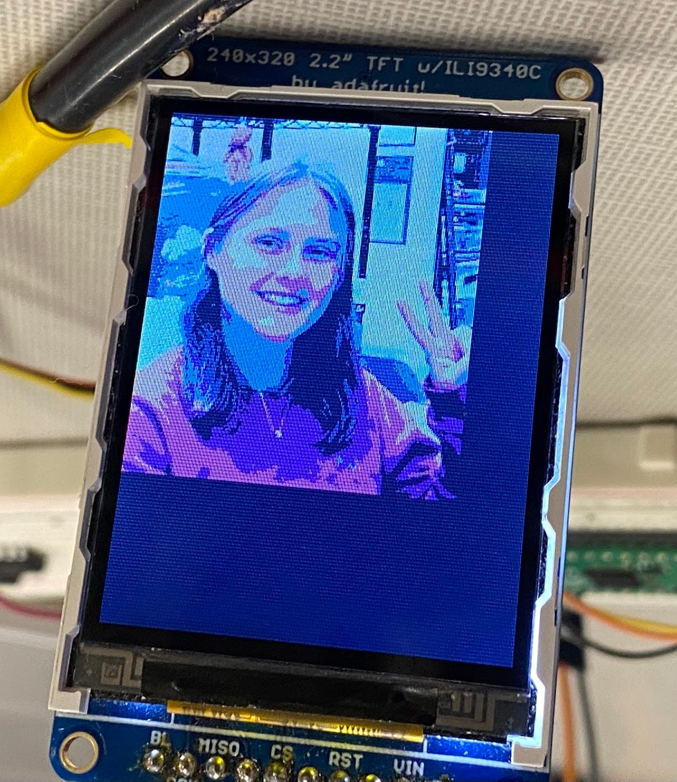
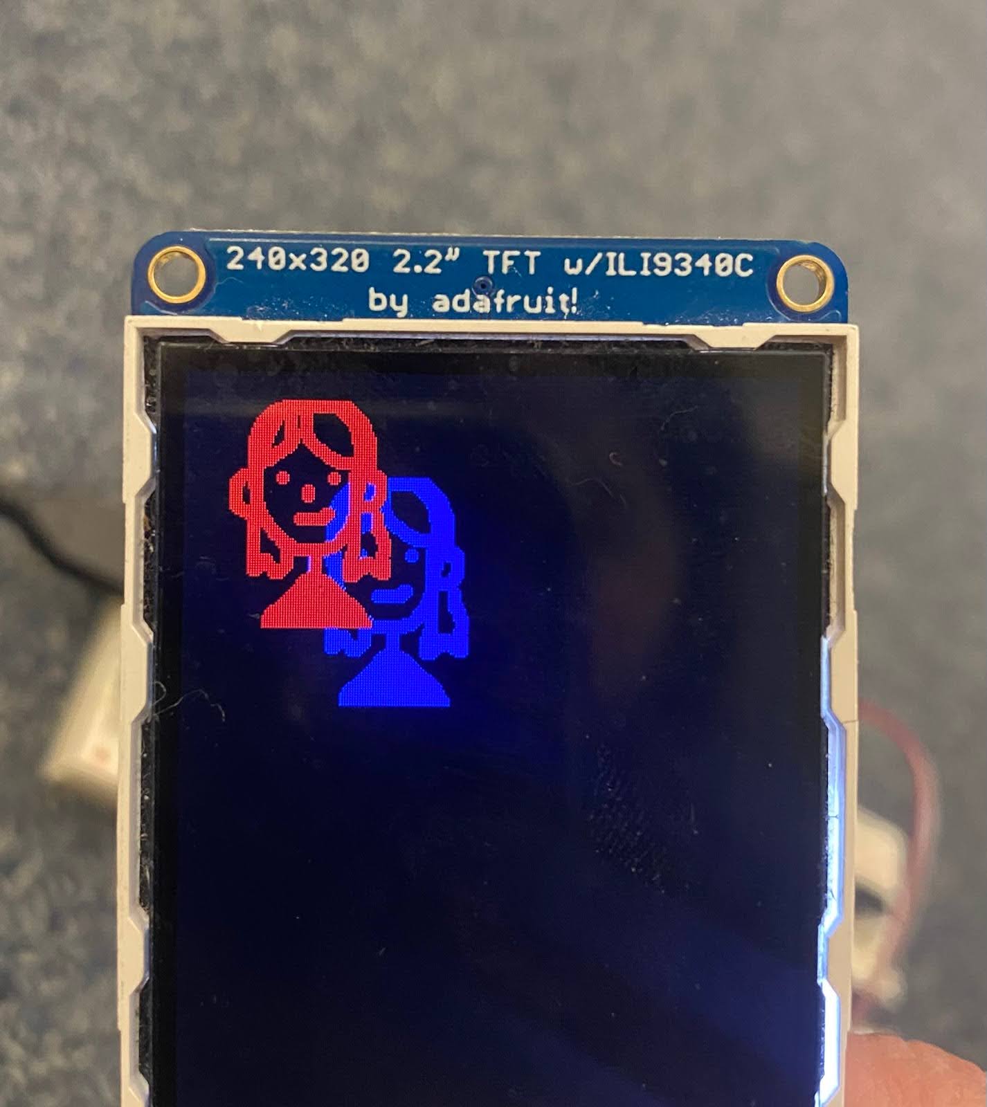 Fig. 6: Caroline's rendition of Rhea layered on the TFT screen using a
sprite canvas.
Fig. 6: Caroline's rendition of Rhea layered on the TFT screen using a
sprite canvas.
We also wrote some additional methods related to graphics: drawing lines with thickness, drawing polygons, and filling polygons with the flood-fill algorithm (later removed because we did not use it). These were useful for drawing the body of the creature based on the output of the physics simulation.
To top off our graphics, we wrote a simple animation control structure which allowed objects, specifically the pet’s face, to be easily animated. We considered both looping and non-looping animations, and allowed for any animation to run at any frame rate (capped by the 30FPS framerate of the animation thread).


For optimization purposes, we were careful not to update the entire screen every frame. Only the sprite canvas is updated at 30FPS, as the soft-body simulation is (almost always) constantly in motion. The UI is updated twice a second, and the general layout (in black) is never redrawn. All assets were created by Caroline using the pixel art software Aseprite.
 Fig. 8: The sprite that covers the screen when your pet dies.
Gameplay
Not too much to say here. We built a small state machine to process button inputs. Because we used those black, square buttons, we had to register input as any change in the button’s pin, instead of just up or down, so our state machine was extremely simple. When a button is pressed and the corresponding animation is not currently playing, an animation plays and a stat is updated. When in the “death” state, any button input resets all statistics and miraculously reanimates your pet.
Physics
The physics protothread uses the most “set” constants that we tune later on to make sure that our simulation is as seamless as possible. The thread begins by initializing everything needed for the simulation to run: vertices and springs. We chose there to be 12 vertices and subsequently 12 springs as well. This is a value that can easily be tuned depending on how fine-grained you want your bounce to be (and overall how “jiggly” you would like your soft body to be). The more springs and vertices you add, the more “jiggly” your soft body is. We did not adjust this value once we chose 12 to be the number of springs, because our creature looked roughly circle without too much overhead as it was. Each vertex is initialized to be around a circle of a fixed radius (we chose 20 units) and the corresponding spring also has the same coordinates. When initializing the springs, we set the vertices by number to make our computations easier. So, vertex_a is set to the same number as the spring (i) and vertex_b is set to be the next vertex (i+1). We also implement wrap around logic to make sure the spring is a complete circle for the last spring. The length of the spring, which is initialized to be in its relaxed state, is the Euclidean distance between the two points.
    // arrange vertices in a circle
    for (int i = 0; i < vertex_count; i++) {
        int x = (int)(radius * sin(i * (2 * M_PI) / 12.) + (right - left) / 2.);
        int y = (int)(radius * cos(i * (2 * M_PI) / 12.) + (bottom - top) / 2.);

        vertices[i].x = x;
        vertices[i].y = y;
        xs[i] = x;
        ys[i] = y;
    }

    //create springs between adjacent vertices
    for (int i = 0; i < vertex_count; i++)
    {
        if (i == vertex_count - 1)
        {
            springs[i].vertex_a = vertex_count - 1;
            springs[i].vertex_b = 0;
            springs[i].len = distance(vertices[vertex_count - 1].x,
             vertices[vertex_count - 1].y, vertices[0].x, vertices[0].y);
        }
        else
        {
            springs[i].vertex_a = i;
            springs[i].vertex_b = i + 1;
            springs[i].len = distance(vertices[i].x, vertices[i].y,
             vertices[i + 1].x, vertices[i + 1].y);
        }
    }
There are several forces acting on your pet at one point in time. The first one we encode is gravity, which affects the force on a vertex in both the x and y directions. We calculate gravity using our accelerometer readings, which helps create the illusion that the simulation obeys the same gravity that we experience. The gravitational force operates based on the equation F = m*g*a as both gravity and acceleration from the IMU are accelerations.
       for (int i = 0; i < vertex_count; i++)
       {
           vertices[i].fx = mass * gravity * -fix2float15(acceleration[0]);
           vertices[i].fy = mass * gravity * -fix2float15(acceleration[1]);
       }
We then calculate the forces on each spring (spring force from Hooke’s Law and the normal force). Hooke’s Law dictates that the force placed upon a spring is proportional to its physical displacement. Once those forces are calculated, we accumulate the force for each start and end point of the spring. Using the coordinates of the start and the end of each spring, we also calculate the normal vectors.
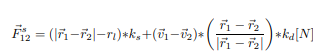 Fig. 9: Hooke's Law.
This is the equation that describes spring linear force, where r1 is position of the first spring point, r2 is a position of second spring point, rl is rest length of the spring length, and ks and kd are spring and damping factors. The code implementation mirrors this equation. The direction of the force is dependent on the sign on the fx and fy terms. The force is subtracted from vertex a because the force itself is calculated pointing from vertex b to a. Thus, vertex a feels the force from vertex b and is pulled towards it. However, the force is added to vertex b because it feels an opposite and equal reaction to the subsequent force from vertex a and feels pushed towards vertex a (Newton’s third law).
          for (int i = 0; i < spring_count; i++)
          {

              float x0 = vertices[springs[i].vertex_a].x;
              float y0 = vertices[springs[i].vertex_a].y;
              float x1 = vertices[springs[i].vertex_b].x;
              float y1 = vertices[springs[i].vertex_b].y;

              float dist = distance(x0, y0, x1, y1);
              // prevent divide-by-zero for too-near points
              if (dist < 1e-6f)
              {
                  springs[i].norm_x = 0;
                  springs[i].norm_y = 0;
                  continue;
              }

              float vx = vertices[springs[i].vertex_a].vx
                - vertices[springs[i].vertex_b].vx;
              float vy = vertices[springs[i].vertex_a].vy
                - vertices[springs[i].vertex_b].vy;

              // hooke's law
              float f = (dist - springs[i].len) * spring_const +
                        (vx * (x0 - x1) +
                         vy * (y0 - y1)) *
                            spring_damping / dist;
              float fx = ((x0 - x1) / dist) * f;
              float fy = ((y0 - y1) / dist) * f;

              // force on starting spring
              vertices[springs[i].vertex_a].fx -= fx;
              vertices[springs[i].vertex_a].fy -= fy;

              // force on ending spring
              vertices[springs[i].vertex_b].fx += fx;
              vertices[springs[i].vertex_b].fy += fy;

              // set normal vectors
              float nx = (y0 - y1) / dist;
              float ny = -(x0 - x1) / dist;

              springs[i].norm_x = nx;
              springs[i].norm_y = ny;
          }
The volume of a ball is calculated using Gauss’s Theorem, which states that an integral taken over a volume can be replaced by one taken over the surface bounding that volume. We can also use V as the body volume, abs(x1 - x2) is an absolute difference of x component of the spring start and end points, nx is the normal vector x component, and dl is our spring constant.
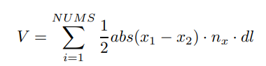 Fig. 10: Gauss’s Theorem.
The code implements the equation exactly, where NUMS is defined to be the total number of springs. This is 12 in our case. We also check in the code if the length of the spring is small (less than 1 * 10 -6) and then make the x and y normalization 0, which means there is no direction of the force.
          float volume = 0.;
          for (int i = 1; i < spring_count; i++)
          {
              // start point
              float x0 = vertices[springs[i].vertex_a].x;
              float x1 = vertices[springs[i].vertex_b].x;

              float y0 = vertices[springs[i].vertex_a].y;
              float y1 = vertices[springs[i].vertex_b].y;

              // end point
              float dist = distance(x0, y0, x1, y1);

              // gauss's with euclidean distance
              volume += 0.5 * fabs(x0 - x1) * fabs(springs[i].norm_x) * dist;
          }
The following pressure force calculation is governed by the following equation, where V is a body volume, A is edge size, P is the pressure value, and n is the normal vector to the edge. In our implementation, we accumulate the forces in the x and y direction for the pressure. This equation’s motivations are as follows. Pressure is force per unit area (P = F/A) and is multiplied by the normal vector for direction. Thus, F = A * P * n. Then, in soft body physics says that the pressure is applied across the whole body, which is why we divide by the volume.
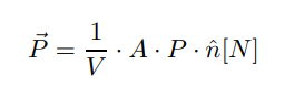 Fig. 11: An expression representing pressure on each vertex.
In the code implementation, we add the force in each direction of the force to vertex a and b because the pressure is meant to push the force outwards. The same force is applied to both vertices because both equally contribute to the pressure as pressure is related to the edges of the soft body not the vertices. We also have a default pressure of 200 if the pressure is calculated to be below 0.00001. To make sure the soft body does not collapse in on itself.
          for (int i = 0; i < 12; i++)
        {

            // start point
            float x0 = vertices[springs[i].vertex_a].x;
            float y0 = vertices[springs[i].vertex_a].y;
            // end point
            float x1 = vertices[springs[i].vertex_b].x;
            float y1 = vertices[springs[i].vertex_b].y;
            float dist = distance(x0, y0, x1, y1);

            float p = dist * pressure * (1 / volume);

            // cap on lower end
            if (is_approx_zero(p))
            {
                p = 200;
            }

            float px = springs[i].norm_x * p;
            float py = springs[i].norm_y * p;

            // apply to forces
            vertices[springs[i].vertex_a].fx += px;
            vertices[springs[i].vertex_a].fy += py;

            vertices[springs[i].vertex_b].fx += px;
            vertices[springs[i].vertex_b].fy += py;
        }
The first part of this code recalculates the velocity (v = f/m * dt = a * dt) and position (pos = v * dt) of the spring based on time intervals, which is based on the derivative equations of motion. The inclusion of this step is to make sure that our soft body accurately changes velocity and position even when it is not bouncing against a wall, and there is nothing to exert force on the soft body. This is the collision code logic where we execute the restitution (or the bounce) from hitting the wall in the other direction. We measure if the vertices exceed the bounds of the wall. If they do and the force is high enough against that wall (x force higher than 1000 for a hit against the left or right wall or y force higher than 1000 for a hit against the top or bottom wall), we call triggerHit() to reduce statistics and change facial expressions. We also ensure that the point values never exceed the bounds of the window once the hit against the wall is checked.
This is the collision code logic where we execute the restitution (or the bounce) from hitting the wall in the other direction. We measure if the vertices exceed the bounds of the wall. If they do and the force is high enough, we to make our creature dizzy.
          float dry;

          // apply all forces, roughly integrating by time
          vertices[i].vx += (vertices[i].fx / mass) * dt;
          vertices[i].vy += (vertices[i].fy / mass) * dt;

          // apply all velocities, roughly integrating by time
          vertices[i].x += vertices[i].vx * dt;
          vertices[i].y += vertices[i].vy * dt;

          // bounce off walls
          if (vertices[i].x > right || vertices[i].x < left)
          {
              vertices[i].vx = -vertices[i].vx * restitution;

              if (vertices[i].x < left)
              {
                  if (fabs(vertices[i].fx) > 1000.0)
                      triggerHit();
              }

              else if (vertices[i].x > right)
              {
                  if (fabs(vertices[i].fx) > 1000.0)
                      triggerHit();
              }
          }

          // bounce off more walls
          if (vertices[i].y < top || vertices[i].y > bottom)
          {
              vertices[i].vy = -vertices[i].vy * restitution;

              if (vertices[i].y < top)
              {
                  if (fabs(vertices[i].fy) > 1000.0)
                      triggerHit();
              }

              else if (vertices[i].y > bottom)
              {
                  if (fabs(vertices[i].fy) > 1000.0)
                      triggerHit();
              }
          }

          // restrict points within the window so we don't get IOOB exceptions
          vertices[i].x = MIN(MAX(vertices[i].x, 0.), right - 1);
          vertices[i].y = MIN(MAX(vertices[i].y, 0.), bottom - 1);
Tuning Parameters for Physics
The constants that were tuned to make sure the Tamagotchi “jiggled” the right amount were the following parameters: spring_const, spring_damping, mass, pressure, gravity, and physics_framerate. The spring_const was increased to be 110 because we wanted compressions to happen less frequently (only if there was requisite force applied). The spring_damping constant was also increased to be 28 because we wanted the springs to be stiffer and not have the springs bounce an unnatural amount. As noted in our demo, the pet will fall towards the current bottom (as in, facing the actual ground) of the screen naturally because there is a gravity constant applied to it. The mass of the pet was increased to 12 (from 10) and gravity to 15 (from 12) to make sure that your pet was more impacted by accelerations (think F=ma!). This increase in mass helped your pet bounce around the screen more "instantaneously." We tuned the pressure to be 12000 to ensure the vertices would not collapse into itself and your pet would not lose its shape. The last constant that we tuned was the physics_framerate to make sure that the physics thread updated as quickly as possible and that it was in coordination with the drawing framerate.
FRAM
We implemented a persistent memory functionality to the tamagotchi so that the state of the tamagotchi’s stats (weight, health, hunger, happiness) can be recovered after disconnecting from power. In order to do this, we implemented a small 32KB I2C non-volatile FRAM breakout. We chose the MB85RC256 model from adafruit, which can run at up to 1MHz I2C rates. We implemented an I2C FRAM driver for the Raspberry Pi Pico. The code reads and writes bytes of a specified length to a given memory address in the FRAM. This code doesn’t handle raw I2C commands and instead uses functions included with “hardware/i2c.h”
mb85rc256.c
In the source file, four functions are defined that set up the FRAM device, test its functionality, read bytes and write bytes.
mb85rc256_init()
A struct MB85RC256 struct is initialized, which assigns the I2C port and device address. We decided to create a struct so that if we potentially wanted other FRAM devices or other I2C devices to be added, all of the addresses related to the specific device would be stored in one place. Each time you would only need to pass a pointer to the struct to access all the information related to that device.
mb85rc256_begin()
The begin function verifies that the FRAM breakout is responding. It writes to a 2 byte address 0x0000 and checks if the FRAM responds to the write. Once the FRAM is verified to be responsive, then the FRAM can have game states written to and read from it.
        mb85rc256_read_bytes((MB85RC256 *dev, uint16_t addr, uint8_t *data,
        uint8_t length)
The read function reads bytes of length defined by “length” from the memory address defined by “addr”. First, the 16 bit address is converted to 2 bytes. The address where the data is read from is sent to the FRAM using the function i2c_write_blocking(). Then the data is read using i2c_read_blocking(). The data is stored in the “data” parameter.
mb85rc256_write_bytes((MB85RC256 *dev, uint16_t addr, volatile uint8_t
        *data, uint8_t length)
The write function writes bytes of length defined by “length” to the memory address defined by “addr”. First, the buffer needs to be constructed such that the first two bytes are the memory address to write to and the following bytes consist of the data to write. Using i2c_write_blocking, the buffer is sent to the FRAM.
mb85rc256.h
In the header file, we defined variables related to the FRAM and defined the MB85RC256 struct. The SDA and SCL pins for the I2C connection are 6 and 7 respectively. We used i2c1 as the channel for communication, since the IMU was using the i2c0 channel. The address specified by the datasheet for the FRAM was 0x50.
Challenges
Along the way, we had some issues with our creature "exploding" due to float arithmetic errors that came up when comparing points that were very, very close. This resulted in vertices having infinite spring forces on them. To fix this, we just ignored forces from nearly-overlapping vertices. We also had to be very careful when considering which parts of the screen needed to be drawn to in the core animation loop, as the TFT driver is not the fastest. This led us to isolate the square enclosure as the only part of the game drawn via sprite canvas. We also had some difficulties getting the buttons to register input normally, as we didn't realize that these specific buttons change the corresponding pin's value each time they are pressed, and assumed that high or low would actually be distinct states. Thank you TA Mahmoud for this revelation.
Hardware Design
The Raspberry Pi Pico has six peripheral devices connected to it: the IMU, the FRAM, the TFT screen, and three buttons. Both the IMU and the FRAM are connected by I2C communication, and the TFT screen is written to via SPI.
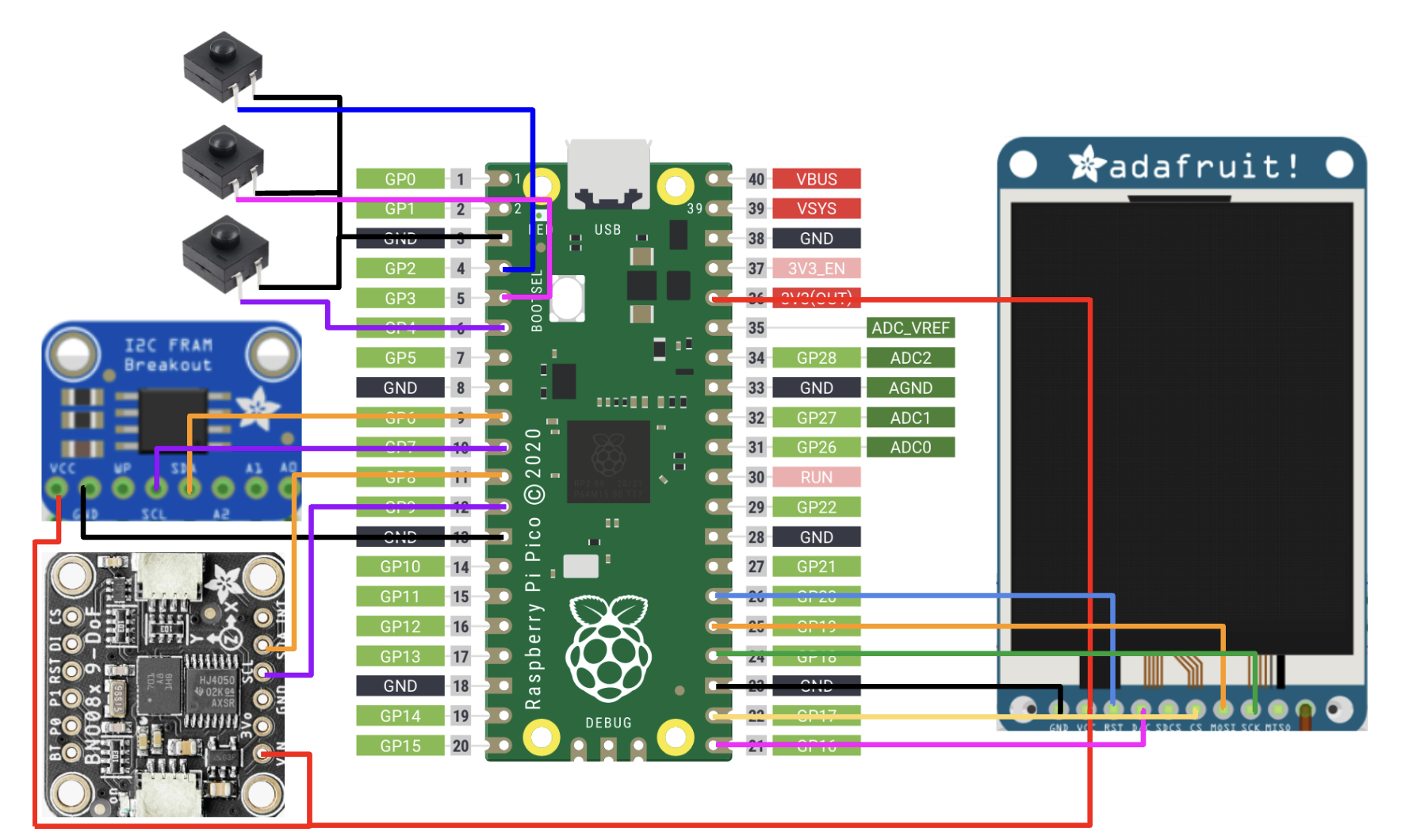 Fig. 12: Our hardware design.
| Device name | Pin connections to RP2040 |
|---|---|
| TFT Screen- MB85RC256 | DC- GPIO 16 CS- GPIO 17 SCK- GPIO 18 MOSI- GPIO 19 RST- GPIO 20 |
| IMU- MPU6050 | SDA- GPIO 8 SCL- GPIO 9 |
| I2C FRAM- MB85RC256 | SDA- GPIO 6 SCL- GPIO 7 |
| Feed button | GPIO 2 |
| Wash button | GPIO 3 |
| Play button | GPIO 4 |
The hardware design for the tamagotchi did not require any additional circuit components. We prototyped on a breadboard until all of the connections were finalized. Once prototyping was completed, we attached all of the peripherals in a solderboard to make the tamagatchi portable and compact. The Raspberry Pi Pico and the TFT screen were soldered on opposite faces of the solderboard for space efficiency. An important note for wiring this device is that since both the IMU and the FRAM use I2C communication, they were connected on separate I2C channels. The IMU used the i2c0 channel and the FRAM used the i2c1 channel.
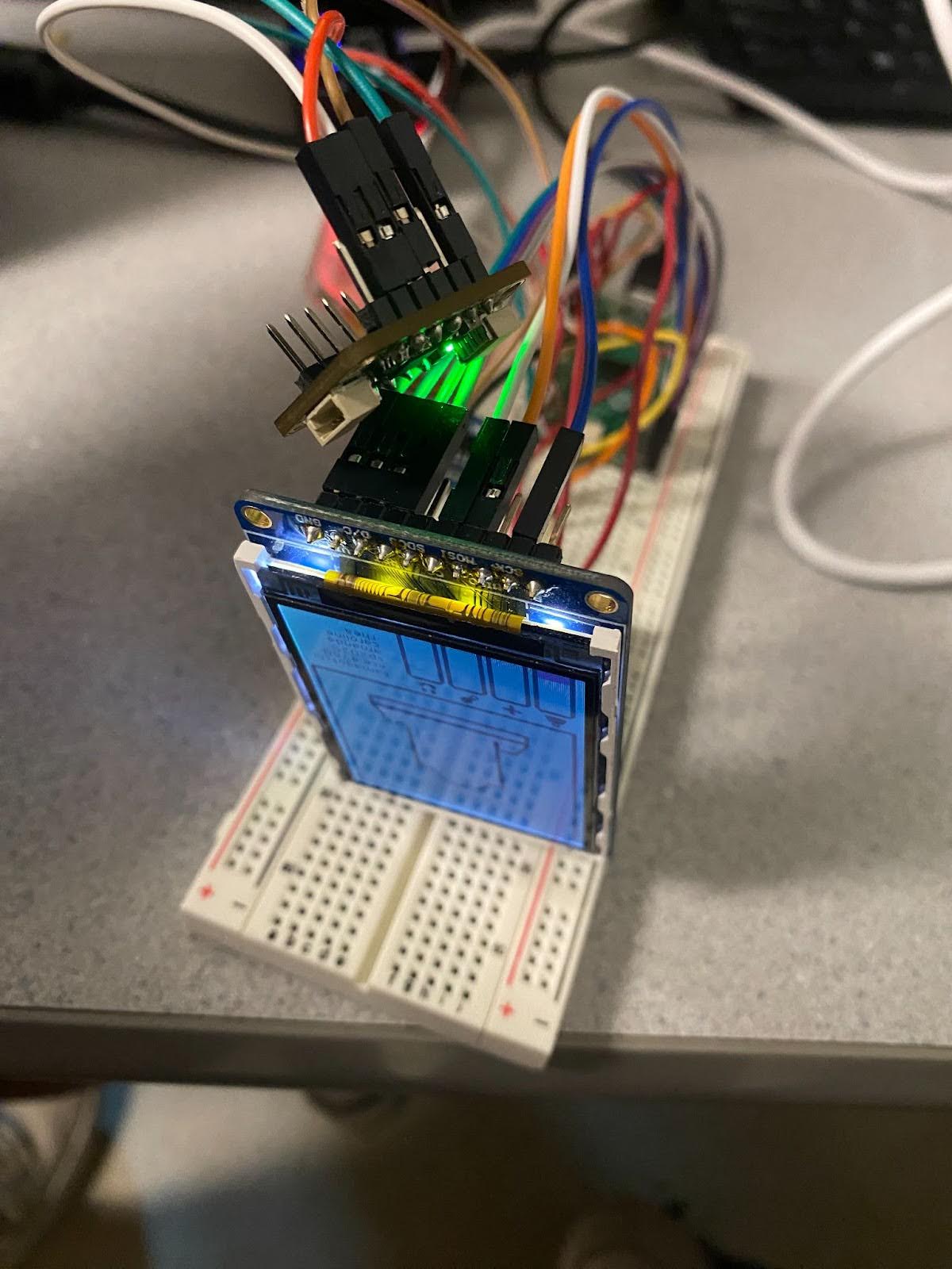
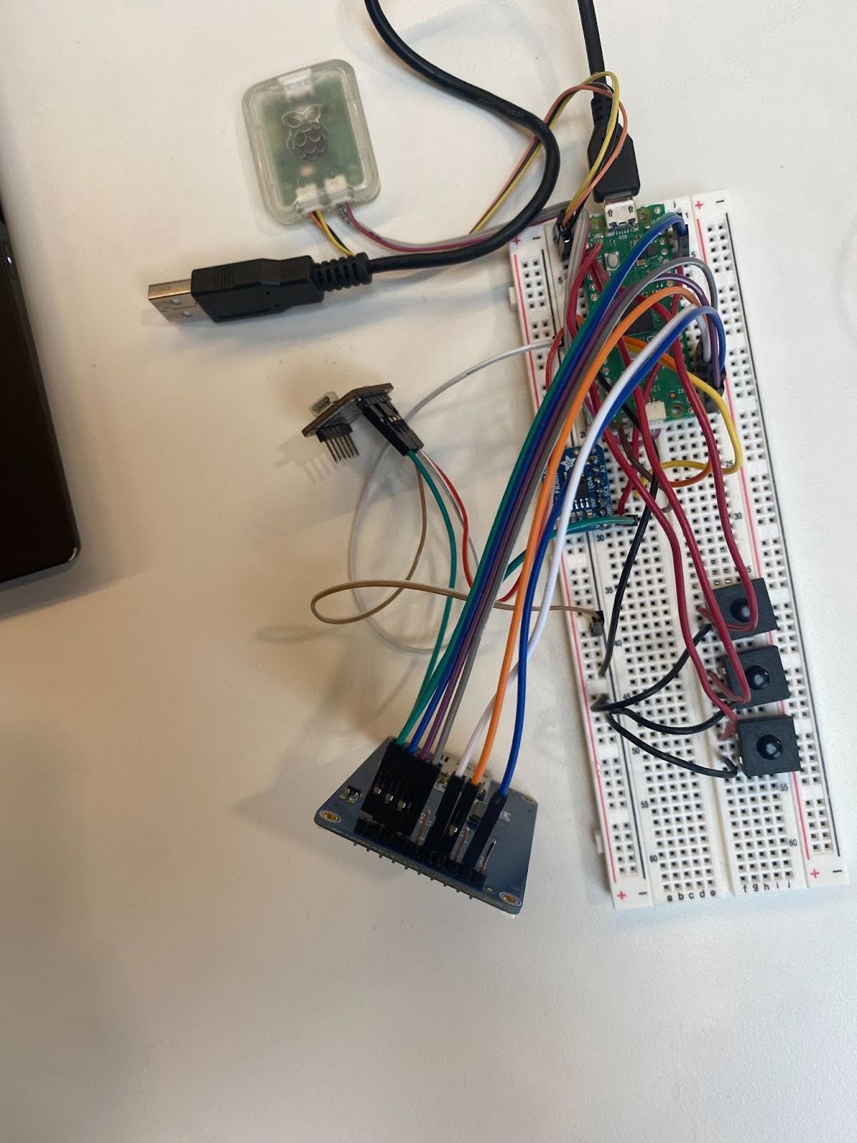
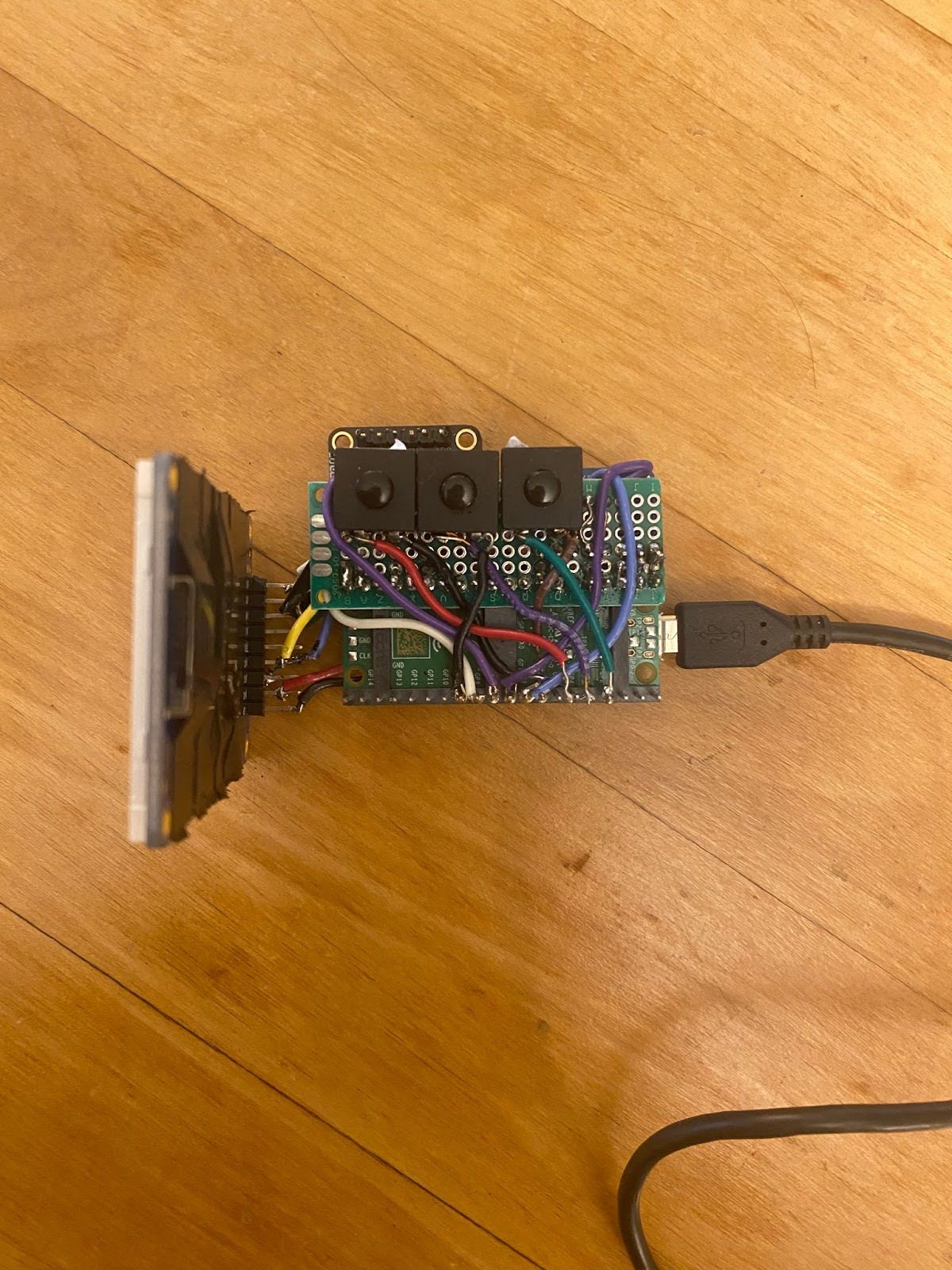 Figs. 16: The solderboard and accompanying wiring.
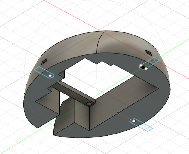
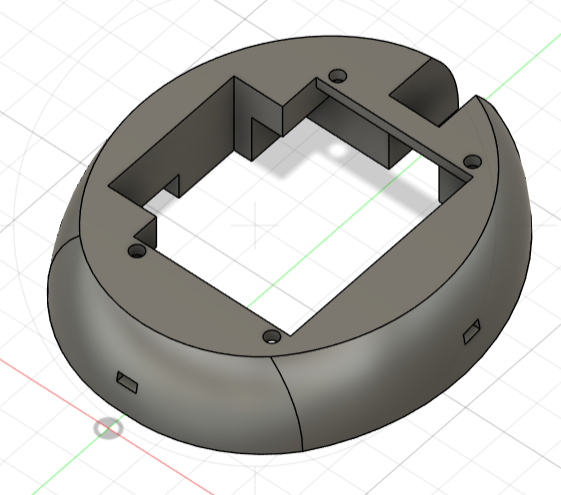
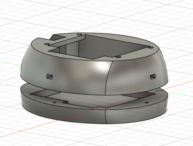
Printing the Case
We develop a 3D printed case for the tamagotchi to improve the user interface. The CAD composed of 2 bodies. The top body held the screen in place, and the bottom body provided extra support and protection to the wiring. The CAD mimicked the original egg-shaped case for the tamagotchi, customizing the size to our project. The design consisted of cutouts for the USB cable, IMU and FRAM components. There are also three cutouts for a nut on the top body. This was to support three 20mm M2.5 screws that would attach the bottom and top parts. Four screw cutouts were also included on the top face to hold the TFT screen in place.
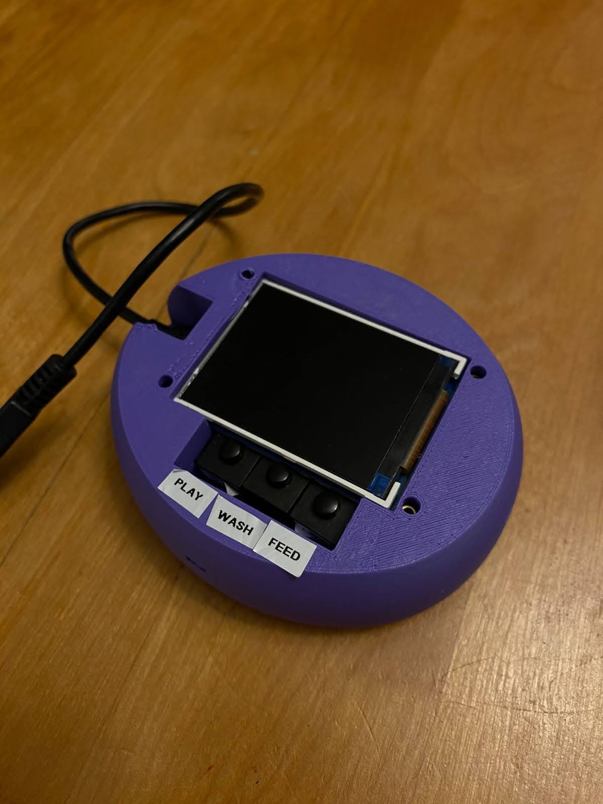
Challenges
When using the solderable breadboard, it was a bit difficult to orient the peripheral devices so that the wiring fit and the device could stay as small as possible. Once parts were soldered and then removed, some wires got cut too short. To re-solder them, we had to extend some wires, which was unideal since exposed wires were just covered by electrical tape. The CAD required a few reprints due to sizing errors and unfamiliarity with 3D print technology. The first print failed, didn’t print, most likely due to selecting incorrect options in the slicing program and failure to add supports. The second print failed since the sizing of the cutout for the screen was too tight. It seemed very close, so we tried to sand down the edges. We tried to force the screen in, and ultimately cracked the screen. As a result, we had to find a new screen and re-solder the connections to the Raspberry Pi Pico. The third print is the final version shown above. In the future, to improve the design of the case further, we would lower the walls surrounding the buttons to make them more accessible and try to reduce the overall size of the body. The internal structure of the case can also be further improved to provide more support to the electronics.
Results
Overall, our tamagotchi with soft body physics simulation runs pretty smoothly. We really tried to optimize our code, so that the game updated almost instantaneously as the user tilted the egg case (which housed the hardware and TFT screen). We did so by putting our threads on different threads and eliminating physics and drawing computations unless absolutely necessary. Unfortunately, our statistics do not always update instantaneously if the user spams the clicky button. If the user takes a second to pause between their presses, then this problem does not occur. With tuning of parameters on our end, we got the tamagotchi physics to react in line with the drawing frame rate. Though it does not update instantaneously if the user shakes the tamagotchi back and forth, your pet will respond really well to gentle tilts of the egg. The drawing updates work as we expected!
There is a certain level of accuracy for the game, but it is partially dependent on the user's inputs. This accuracy is a feature of the gameplay and our tuning. The accuracy looks like the reaction time of your pet on the screen when it gets tilted and the buttons responding. Though we initially encountered issues with the responsiveness and the buttons, we were able to resolve both through tuning and reading the data sheet.
We enforced safety in our design through soldering and the 3D printing of our egg-shaped case. All of our additional components (such as the IMU and the buttons) were soldered directly to a protoboard or attached to the RP2040. This was done to ensure that all the wiring stayed intact while the user shook the egg around. These wires and electronic components were housed within the egg-shaped case, which meant that the user did not have to worry or look at any of the wires present for the system. For accessibility purposes, the buttons were placed next to the TFT screen and labelled. So, the user knows which buttons correspond to which actions. There was a clear notch at the top of the case to allow for the micro-usb wire that powers the RP2040 to pass through. The user mainly interacts with the buttons and observes the actions on the TFT screen.
The TTC is very usable and intuitive for others to understand as most people have played with some sort of virtual pet, even if it is not exactly a Tamagotchi. Thus, most players of our game already knew the basic premise of the game from pop culture. Though there is no instruction screen, the user can easily pick up on what each action does by observing how your pet responds as there are only three buttons and each is labeled. Once the user presses a button, your pet should experience the action and the statistic bars at the bottom should increase or decrease accordingly. Our game is very user friendly because the rules are primarily centered around having fun with your creature. One big change that we could have made was to make the physics smoother and have the creature be able to bounce around the screen quicker instead of slowly sliding around like it does currently. We observed and tested our tamagotchi game through qualitative means, such as playing with the game ourselves and having multiple people who were unfamiliar with our game play with your pet. Everyone was able to get familiar with the game quickly as there are very few rules and have fun interacting with the pet!
Conclusion
We were hoping to have our simulation be a little more sensitive to quick changes in acceleration. For example, we were thinking that the creature could slam up against the walls when a user shook the device. However, we discovered that running the physics simulation at a faster rate would cause its animation to look choppy and overly-jiggly, so we decided to stick with a smoother tuning. We also were not able to find a nice way to fit batteries into our handheld design, which would have been necessary for the TTC to be truly portable.
Besides that, to roughly quote Professor Adams, our implementation is nearly identical to our initial proposal, but for the addition of soft body physics. In that way you could say we exceeded the expectations that we set in our project proposal.
If we were to design this project again, we might start on the CAD for our case earlier, as our final product had the buttons set way back to the point that they were difficult to access. We would also find a way to incorporate battery power without making the device too large, so it could be fully portable. On the software side, we could spend more time tuning the physics simulation to be more sensitive to IMU input and experiment with different spring configurations. We could also rewrite the game’s UI to more closely resemble the original device’s.
Our physics simulation code is roughly adapted from both Maciej Matyka’s original paper and Nathaniel Brookes’s Javascript implementation of it (see Appendix E for both). Both of these projects are open-source and in the public domain. We also used Parth Sharma’s TFT driver, which was written for this class and provided to us by Professor Adams.
Although the design and implementation is entirely our own, we cannot patent this project as the name “TAMAGOTCHI” and the concept of an egg-shaped virtual pet are trademarked by Bandai. We aren’t seeking to sell this device, and are only making one copy. Because we made the TTC to further our education, we believe this project falls under Fair Use.
We had a lot of fun working on this project, and are proud to present a fully functional and good-looking device at the end of the day. Special thanks to Professors Land and Adams and the ECE4760 TAs for their patience, Zoe Matzkin (‘27) for her excellent modelling, and Charles Yang (‘26) for the last-minute CAD aid.
 Fig. 22: Selfie taken after our final demo. From left to right:
Professor Adams, Rhea, Caroline, and Amanda.
Fig. 22: Selfie taken after our final demo. From left to right:
Professor Adams, Rhea, Caroline, and Amanda.
Appendices
Appendix A (Permission)
The group approves this report for inclusion on the course website. The group approves the video for inclusion on the course youtube channel.
Appendix B (Code)
Our code is available on Github.
Appendix C (Schematics)
Refer to the Hardware Design section for schematics.
Appendix D (Work Distribution)
All of us were involved in creating each aspect of this project. We worked together to assemble the hardware and software for this project. There were some parts that we did separately. Amanda worked on soldering the extension board, creating the case, and persistent memory code implementation. Caroline worked on all the animations and drawing logic and created this web page. Together, Rhea and Caroline worked on the implementation of soft body physics. Other than these parts, almost all of the project and debugging were done together with all members in the lab. This report was written by all three members.
Appendix E (References)
Course References:- ECE 4760 Course Website (Lab 3 IMU Code)
- "How to implement a pressure soft body model" by Maciej Matyk
- Nathaniel Brookes's implementation of the above: source and website