Vision-Guided Ball Catcher

Introduction

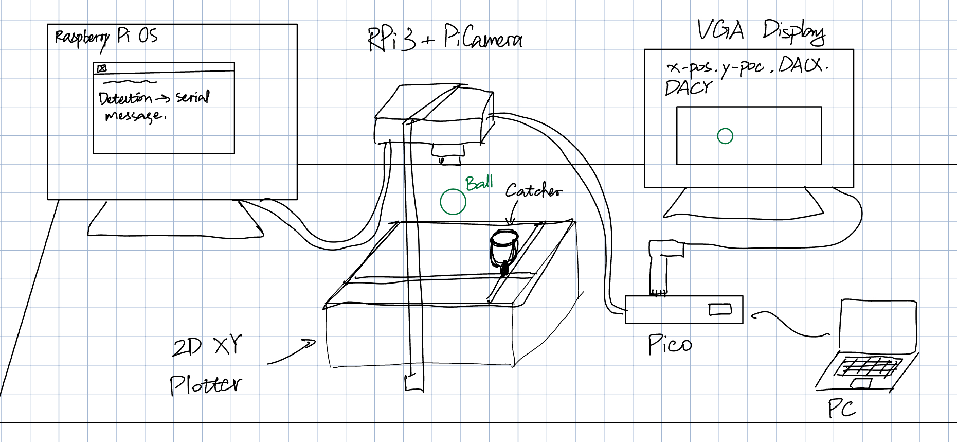
A real-time vision-guided ball-catching system that integrates sensing, computation, and actuation to react to fast, dynamic events, in this case a flying ball.

This reactive ball-catching machine was developed by Yusheng Chen and Shashank Chalamalasetty as the final project for ECE 5730 at Cornell University in Fall 2025. The system is capable of detecting a moving ball, predicting its motion, and driving a two-axis plotter to intercept it in real time. A top-down camera is used to track the ball's position across consecutive frames, and the resulting data is processed by a computer vision pipeline running on a Raspberry Pi 3 via a Picamera. The estimated state of the ball is then communicated to a deterministic, real-time control system implemented on a Raspberry Pi Pico, which commands the plotter to move toward the predicted landing position as quickly and accurately as possible.

The primary goal of this project is to simulate human hand–eye coordination during object catching using a machine-driven system. This responsiveness-oriented design explores how embedded systems coordinate sensing, computation, and actuation under strict timing constraints, specifically before the ball lands. Due to hardware limitations and engineering trade-offs, the project does not aim to achieve perfectly accurate physical modeling. Instead, it emphasizes successful system integration, real-time responsiveness, effective task partitioning between devices, reliable inter-device communication and control, and practical debugging and visualization techniques.

High Level Design

Rationale and sources of idea

The core idea investigated in this project is responsiveness. The motivation comes from observing how humans handle fast and uncertain physical interactions with little explicit computation. When catching a falling or thrown object, humans rely on incomplete sensory information, make rapid predictions, and continuously adjust their motion, rather than solving a precise physical model. This behavior highlights an important principle in real-world systems: effective performance often emerges from timely, approximate decisions instead of exact calculations.

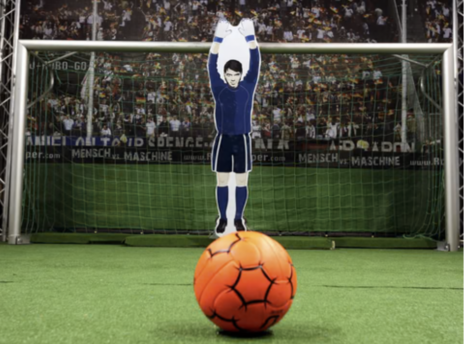
In practice, many engineered systems similarly prioritize responsiveness and robustness over optimality. For example, industrial sorting lines identify and divert objects within fractions of a second without fully reconstructing their shape. Automated door systems respond to human motion using simple sensors without detailed prediction of intent. In the context of this project, a closely related inspiration is the concept of a robotic goalkeeper, which must intercept a flying ball before it enters the net using limited sensing and short reaction times.

Background Math

The mathematical components used in this project are intentionally lightweight in order to minimize computational burden and achieve fast system response. With ball detection and catcher actuation distributed between the Raspberry Pi computer and the Raspberry Pi Pico microcontroller, two key mathematical tools are employed: a geometric measure for object detection on the vision side and a digital filtering technique for noise reduction on the control side.

On the vision processing side, object detection relies on a circularity metric to identify the ball among candidate contours extracted from each frame. For each detected contour, circularity is computed using the formula.

where A and P are the area and perimeter of the region, respectively. This dimensionless metric approaches unity for perfect circles and decreases as the shape becomes less circular. By thresholding this value using a minimum circularity parameter, the system effectively filters out irregular shapes caused by noise or background artifacts.

On the embedded control side, a digital low-pass filter is applied to the received position measurements to reduce noise and prevent abrupt actuator commands. In practice, raw data often contains noise introduced by sensor imperfections and inherent mechanical or electrical fluctuations in the system. In this project, the primary noise affecting the Pico originates from the PiCamera connected to the Raspberry Pi computer. Without appropriate digital filtering, these measurements would exhibit instability, obscuring the underlying motion trend and degrading the accuracy of subsequent computations.

To address this issue, the filter is implemented as an evolving weighted average between the raw measurement and the previously smoothed value. In particular, a first-order infinite impulse response filter is used, which can be expressed iteratively as

with an identical formulation applied to the y coordinate. Here, x_raw[k] represents the current measurement, x_filtered[k] the filtered output, and α a smoothing coefficient between zero and one. This digital filter attenuates high-frequency noise while preserving the overall motion trend.

Logical Structure

The logical flow of each ball-catching attempt operates as a closed-loop pipeline that converts visual observations into real-time actuator commands. At a high level, as the ball moves through the workspace, its position is repeatedly measured by the camera and processed to produce updated predictions of its future location. These predictions are continuously transmitted to the embedded controller, which adjusts the motion of the catcher in response.

At a more detailed level, the process begins with sensing, where a top-down camera captures images of the workspace at 30 frames per second. Each frame is processed on the Raspberry Pi 3 to detect the ball and extract its position within the camera's field of view. The resulting position data is packaged and sent to the Raspberry Pi Pico over a serial communication channel.

Upon receiving this data, the Pico applies digital filtering to stabilize the measurements and performs additional processing, including estimating the ball's motion and generating a short-term prediction of its future location. This prediction yields a target landing position, which is mapped to actuator commands for the two-axis plotter. The actuator commands drive the catcher toward the predicted interception point while maintaining smooth and responsive motion. By separating vision processing from control execution, the system prevents computationally intensive tasks from interfering with time-critical actuation.

Hardware and Software Trade-offs

A primary architectural trade-off in this project is the separation of responsibilities between the Raspberry Pi 3 and the Raspberry Pi Pico. The Raspberry Pi runs a full operating system and supports camera interfacing and computer vision libraries, making it well suited for image processing in Python with extensive library support. However, this flexibility comes at the cost of nondeterministic timing and variable latency due to operating system overhead. In contrast, the RP2040 on the Pico provides deterministic execution and low-latency response, which are critical for real-time actuator control, but it has limited computational resources for visual processing. In line with the project's emphasis on Pico-based embedded design, the Pi is therefore responsible only for extracting ball state information from the PiCamera, while all signal processing and motion control tasks are assigned to the Pico. This division balances computational capability with real-time reliability.

Another important trade-off involves the relationship between camera placement and mechanical actuation limits. Experimental testing showed that the two-axis plotter requires approximately 0.6 seconds to move across the workspace, which corresponds to a free-fall distance of about 1.77 meters in the absence of communication and processing delays. If the estimated Pi-to-Pico communication latency of roughly 0.05 seconds is assumed, the required detection height increases to over 2 meters to allow sufficient reaction time. Practical constraints such as laboratory space and field-of-view limitations make this configuration less reliable. As a compromise, the camera is placed approximately 1 meter above the workspace, and the experimental setup emphasizes controlled ball release rather than unpredictable throws. This approach maintains the responsiveness-focused nature of the project while remaining within mechanical and sensing constraints.

Hardware & Program Design

Hardware Details

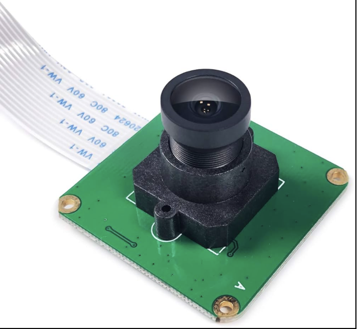
Pi-Camera-OV5647

The vision pipeline uses a Raspberry Pi-compatible camera module based on the OV5647 image sensor. The camera is equipped with an M12 wide-angle lens, providing a sufficiently large field of view to cover the entire plotter workspace from an overhead mounting position. The camera is connected to the Raspberry Pi 3 via the CSI ribbon cable interface. The Pi computer alongside the camera are mounted approximately 1 meter above the workspace in a fixed top-down configuration.

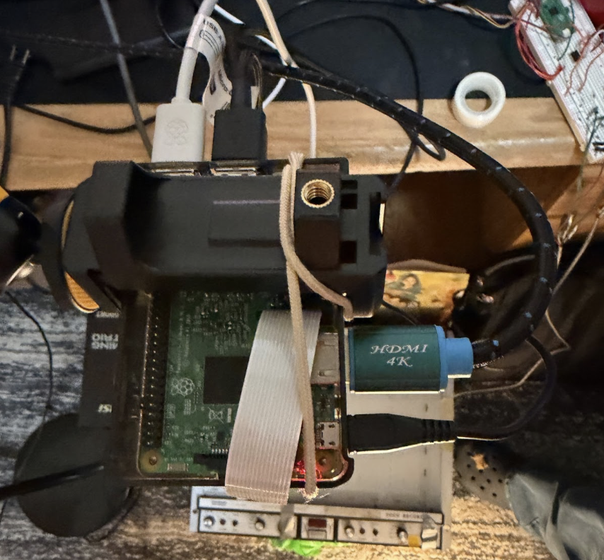
Raspberry Pi 3

Lightweight computer responsible for image acquisition and ball detection. It interfaces directly with the camera module and runs a Python-based vision pipeline using standard computer vision libraries. The Pi extracts the ball's position from each frame and transmits this information to the embedded controller via serial communication channel. is not used for any time-critical control tasks.

Raspberry Pi Pico

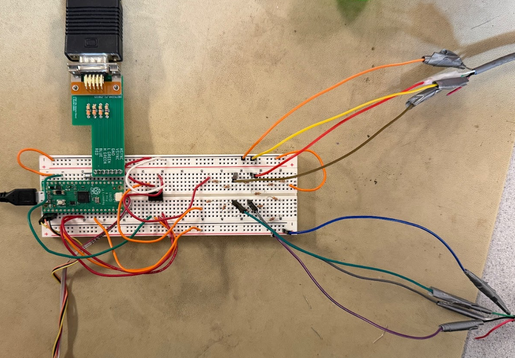
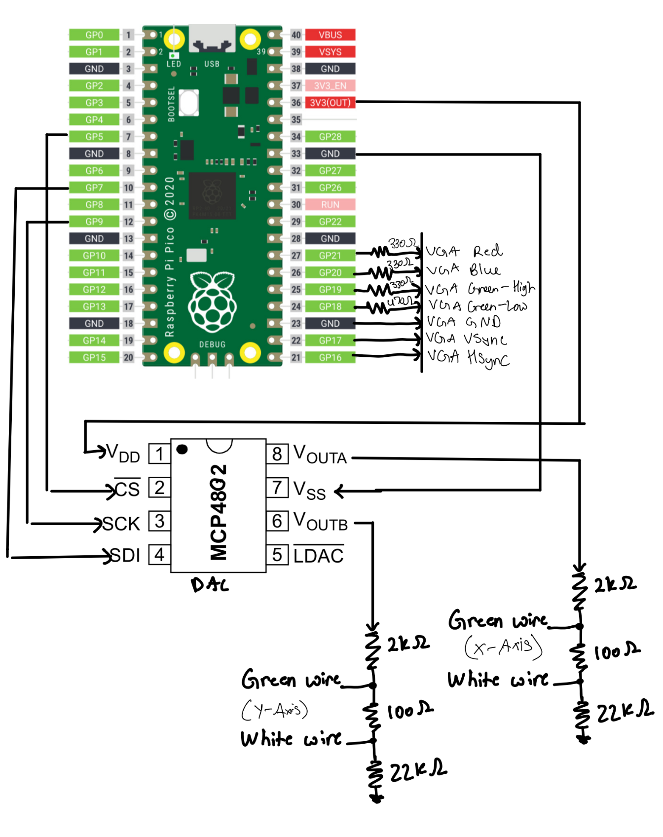
The Raspberry Pi Pico, based on the RP2040 microcontroller, serves as the central real-time control unit of the system. It receives ball position data from the Raspberry Pi via a serial communication interface and is responsible for driving the plotter end effector to the appropriate position.

The Pico generates plotter control signals through two passive voltage divider circuits, one for each axis, which will be described later. Upon receiving a new ball state update, the Pico performs all signal conditioning, short-term prediction, and actuator command generation. All control logic is implemented in C to ensure predictable execution timing and deterministic behavior. In addition to control tasks, the Pico renders a VGA-based graphical interface that displays real-time system state information, including the latest position of the ball. The Pico's low interrupt latency and deterministic execution make it well suited for handling timing-sensitive control and its dual-core capability enables visualization tasks in parallel.

Voltage Divider Circuit (Breadboard Circuit)

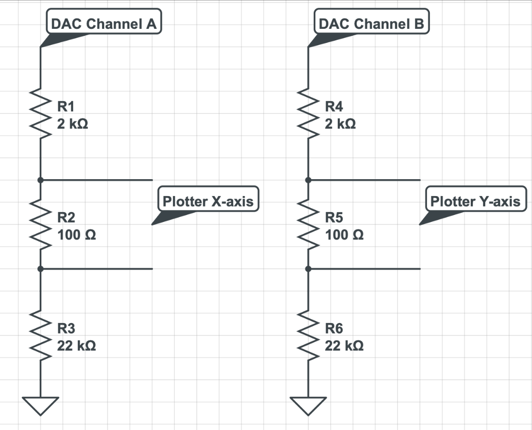
The interface between the Raspberry Pi Pico and the XY plotter is implemented using a passive resistive ladder for each axis, as shown in the schematic. Each DAC channel from the Pico drives a series chain of resistors connected to ground. For the X-axis, DAC Channel A feeds a ladder consisting of a 2 kΩ resistor (R1), a 100 Ω sense resistor (R2), and a 22 kΩ resistor (R3). An identical structure using DAC Channel B and resistors R4-R6 is used for the Y-axis.

Rather than measuring a single node voltage relative to ground, the plotter’s analog input for each axis is connected differentially across the 100 Ω resistor in the ladder. As a result, the plotter senses the voltage drop across this resistor, which is proportional to the current flowing through the entire resistor chain. This current is controlled directly by the DAC output voltage and the total resistance of the ladder.

Inspiration came from the voltage divider circuit of this Latte Art Machine project , but the resistance values are determined by trial and failure.

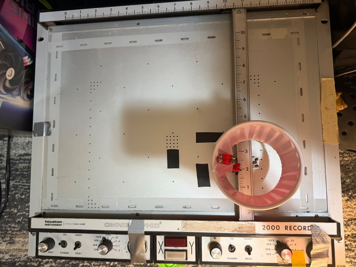
Bausch & Lomb Recorder 2000

This is a legacy precision plotting device originally designed for laboratory and optical instrumentation applications. The plotter provides two orthogonal, independently controlled linear motion axes and accepts analog control voltages to command the X and Y positions of its end effector. Because the plotter does not provide direct position feedback to the controller, accurate operation relies on careful calibration of the voltage-to-position linear mapping and repeatable mechanical behavior.

In this project, the catcher mechanism is mounted at the plotter's end effector, allowing it to translate across the workspace to intercept the ball. The plotter's analog control interface makes it well suited for integration with microcontroller-based systems, as position commands can be generated directly from scaled DAC outputs.

Software Details

Pi Feature: Calibration Window

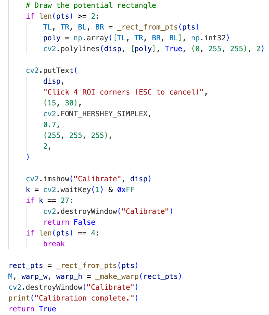
Within the vision processing pipeline, the state of the robot is ideally characterized by pixel coordinates in each frame, which requires a clear and consistent definition of the coordinate origin at system startup. Accordingly, the first operation performed during initialization on the Raspberry Pi is manual definition of a region of interest. The program displays a live camera feed and prompts the user to select four corner points corresponding to the boundaries of the plotter workspace. These points are then used to compute a perspective transformation that maps the camera view into a rectified top-down coordinate frame. This calibration step ensures that all subsequent ball position measurements are expressed in a consistent and repeatable coordinate system.

Pi Feature: Ball Detection Using Color Map and Circularity Checking

Ball detection on the Raspberry Pi is performed using a combination of color-based segmentation and circularity checking aforementioned. Each captured frame is first converted into an appropriate color space, and a color mask is applied to isolate pixels corresponding to the ball. For this project, we use a purely green ball for high contrast. Next, candidate contours are filtered using a circularity metric computed from contour area and perimeter, allowing the system to reject irregular shapes and background artifacts. The shape that best resembles the geometry of a circle and falls into the defined threshold is identified as a “ball”.

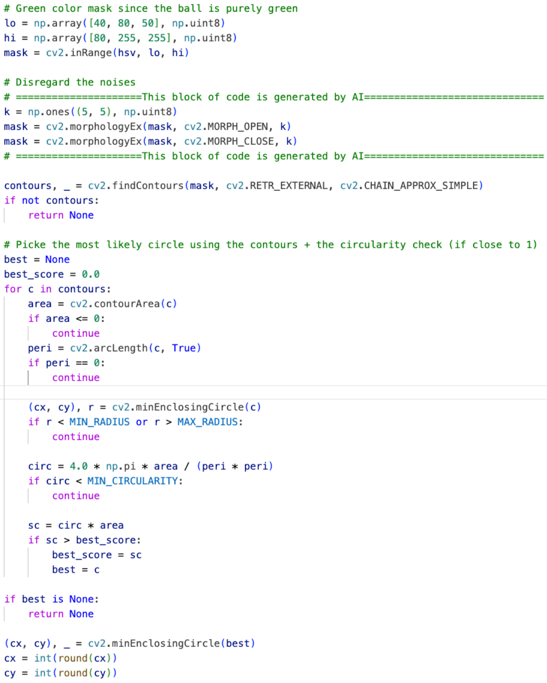
Ball detection logic uses HSV color thresholding, contour extraction, and minimum enclosing circle, inspired by the PyImageSearch "Ball Tracking with OpenCV" tutorial .

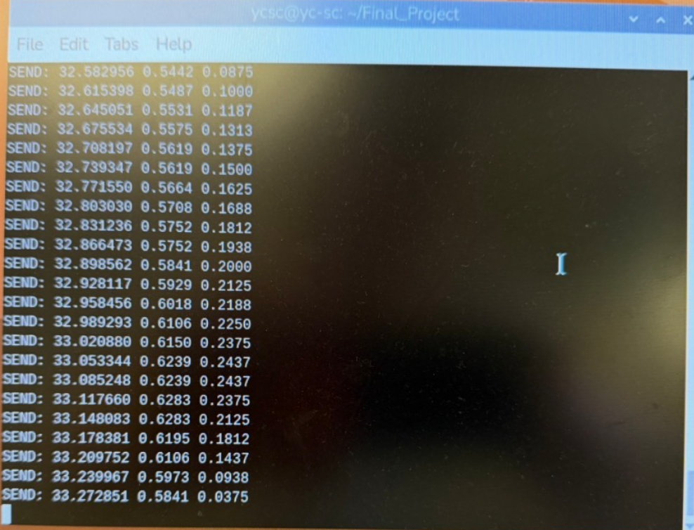
Pi Feature: Timestamped Serial Communication Format

Once a valid ball position is detected, the Raspberry Pi transmits the ball state to the Pico using a lightweight serial protocol. Each message is formatted as a single line containing a timestamp and the normalized x and y coordinates of the ball, where the workspace width and height are treated as unit length, in the form “timestamp x_coord y_coord”. Including an explicit timestamp allows the Pico to account for irregular update intervals, discard consecutive messages with negligible change to improve efficiency, and estimate motion based on actual time differences between measurements. This design improves tolerance to communication latency and variability introduced by operating system scheduling.

Pico Feature: Short-Term Motion Prediction

Once the position of the ball is sensed, there is an inherent delay before the corresponding actuation can occur due to communication and mechanical response time. As a result, attempting to intercept the ball based solely on its current measured position would consistently result in a delayed response. To address this issue, the Pico computes a short-term prediction of the ball’s future position using the timestamped data received from the Raspberry Pi, thereby compensating for both communication and actuation latency.

In this project, the Pico maintains a history of the three most recent ball state updates. For each actuation cycle, a linear extrapolation is performed using the two most recent measurements to predict the ball’s position a short time step into the future. By doing so, the plotter is able to react proactively to where the ball is expected to be, rather than where it was last observed. At the same time, because new measurements continuously update the prediction, the system retains the ability to correct its motion when the latest observation deviates from the predicted trajectory.

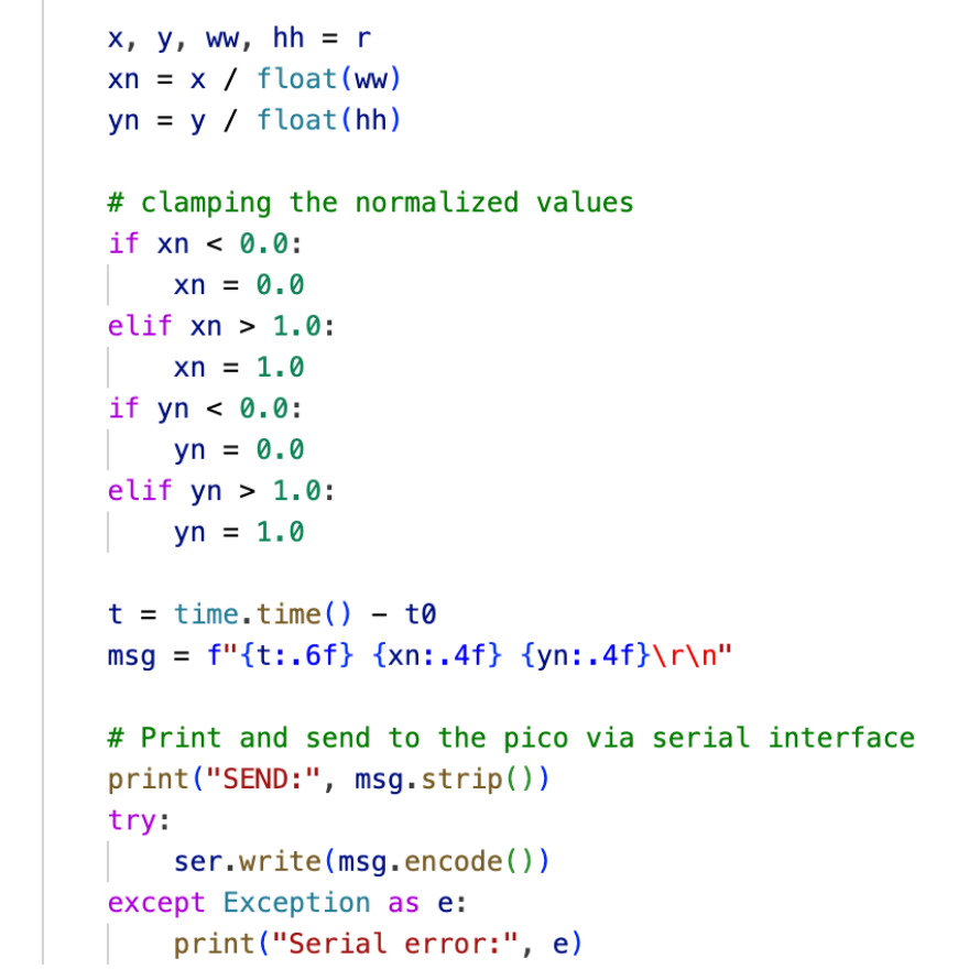
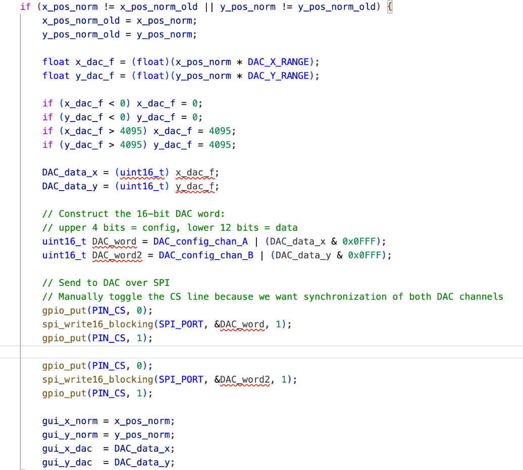
Pico Feature: DAC Output to Plotter Position Mapping

The final stage of the control pipeline on the Raspberry Pi Pico is the conversion of normalized position commands into analog control voltages for the XY plotter. This is implemented using an external dual-channel DAC (MCP4822) driven over SPI. Each actuation update generates one command for the X axis and one for the Y axis, which together define the desired end-effector position.

Normalized position values received and processed by the Pico are linearly mapped to DAC codes within a predefined range. This linear mapping was selected based on experimental characterization of the plotter response using an external laboratory power supply, which demonstrated an approximately linear relationship between applied control voltage and plotter displacement over the usable workspace.

Before transmission, all DAC commands are explicitly clamped to valid bounds to prevent out-of-range voltages that could drive the plotter beyond its mechanical limits. DAC updates are sent over SPI, with each channel packaged as a 16-bit command word containing both configuration bits and the desired output value. Chip-select is controlled manually in software to ensure deterministic framing and synchronized updates across both channels.

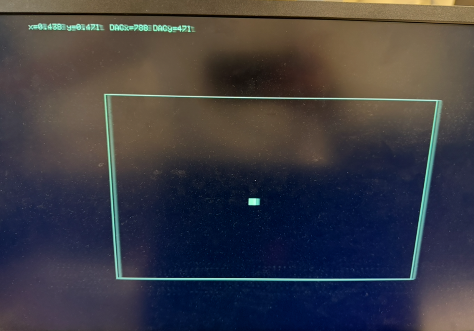
Pico Feature: VGA Graphical User Interface

In addition to generating control inputs, the Pico renders a VGA-based graphical user interface that displays real-time system state information. This includes the incoming serial message and the corresponding DAC output values for the X and Y channels, shown as text in the top-left corner of the display. A rectangular region representing the calibrated workspace is also drawn, within which a white marker indicates the current sensed position of the ball.

From a system design perspective, the VGA rendering workload is executed entirely on core 1 of the RP2040, while core 0 is dedicated to signal processing and actuation command computation. Synchronization between the two cores is achieved through shared state variables written by core 0 and sampled by core 1 at the beginning of each display refresh cycle. This separation exploits the dual-core architecture of the RP2040 to realize parallelism and ensures that visualization tasks do not interfere with timing-sensitive control operations.

Things Tried but Did Not Work

Several approaches were explored during development that proved unreliable or impractical for the final system. On the vision side, early attempts to perform ball detection using fixed color thresholds without additional geometric filtering resulted in frequent false positives under varying lighting conditions and background noise. These approaches were highly sensitive to illumination changes and required constant retuning, which motivated the introduction of circularity-based filtering to improve robustness.

On the embedded control side, initial attempts to directly map GPIO output signal levels to the physical position of the plotter end effector without repeated calibration led to inconsistent behavior. Mechanical variation and assembly tolerances caused noticeable drift in the voltage-to-position relationship, making a one-time calibration insufficient. This demonstrated the necessity of performing calibration during each system setup.

Serial communication between the Raspberry Pi and the Pico also presented challenges. Initial implementations did not enforce strict end-of-line detection and assumed regular update timing. In practice, this led to cases where incomplete or concatenated messages were parsed on the Pico, causing the plotter to move in a periodic and seemingly random manner. This behavior was further undermined by automatic serial buffer flushing, which occasionally caused loss of synchronization between transmitted data and control commands. These issues ultimately motivated tighter message formatting and more robust parsing logic in the final design.

AI Discussion

Artificial intelligence tools were used selectively during the development of this project as an assistive resource. All high-level system architecture, algorithm selection, hardware interfacing decisions, and control logic were designed and implemented by the project authors. AI assistance was limited to generating scaffolding code patterns, refining syntax, and performing sanity checks, with the goal of reducing development overhead rather than replacing engineering judgment.

On the Raspberry Pi side, AI assistance was primarily used as a reference tool for identifying relevant library methods and standard usage patterns. In particular, it was used to help locate and construct common OpenCV operations such as morphological filtering calls and basic rendering utilities for user feedback during calibration, as well as perspective transform boilerplate. AI tools also suggested general performance optimizations, such as reducing image resolution to improve processing speed, which informed the decision to temporarily downscale the calibrated region during ball detection. However, the underlying vision pipeline, including ball detection logic, coordinate normalization, and serial message formatting, was designed and implemented manually. The circularity metric, threshold selection, and scoring logic were chosen based on mathematical reasoning and iterative experimental testing rather than AI generated suggestions.

On the Raspberry Pi Pico side, no AI generated code was used for control logic, real time processing, inter core scheduling, or hardware interfacing. The Pico firmware is adapted from publicly available Cornell ECE4760 reference code by V. Hunter Adams, as stated in the file header, including the protothreads framework and VGA graphics infrastructure. All additional functionalities and modifications, including serial parsing, timestamp handling, digital filtering, short term motion prediction, deadband logic, DAC configuration, SPI communication, manual chip select control, semaphore based synchronization, and dual core task partitioning, were authored, tested, and debugged by the project team. AI tools were used only minimally for syntax verification or conceptual sanity checks, since correct hardware timing behavior required direct reasoning and hands-on experimentation.

Throughout development, AI tools were occasionally consulted for documentation lookup or alternative ways to express existing logic. All AI generated suggestions were carefully reviewed and incorporated only when they aligned with the experimental observations.

Results of the design

Test Condition

The combined software and hardware design resulted in a system that is responsive, observable, and relatively easy to operate. The setup process is straightforward, and the calibration workflow on the Raspberry Pi makes defining the workspace intuitive. The addition of a VGA display driven by the Pico significantly improves system observability by providing real-time feedback on the interpreted ball position and corresponding plotter commands. This feature proved especially valuable during debugging and calibration, as the plotter head is sensitive to loose connections on the breadboard. Even minor wiring issues can skew the end-effector position or alter movement scaling. The VGA display allows such issues to be quickly identified and corrected.

Several analog knobs on the plotter control the input gain and positional offset of the end effector. These parameters directly affect how the analog control signals generated by the Pico translate into physical motion. Proper calibration of these knobs is necessary for accurate operation and would be difficult to perform reliably without visual feedback. With the VGA display providing a clear indication of the expected plotter position, calibration becomes significantly more manageable. Once the basic behavior of the plotter controls is understood, the system is easy to set up and use.

Speed and Accuracy

In terms of speed and accuracy, the system performs well when tracking a ball that is held and moved by hand within the workspace. When the ball is moved to a new location and held stationary, the plotter head follows closely and settles directly beneath the ball. While precise numerical error metrics were not measured, qualitative testing during demonstrations showed that the closed-loop response is smooth and stable, with minimal hesitation or jitter under normal operating conditions. This confirms that the vision pipeline, communication scheme, and control logic operate effectively in real time.

Safety Considerations

Safety considerations are enforced primarily through software-level constraints. Throughout the control pipeline, normalized position values are clamped to valid bounds before being processed or transmitted. On the Pico side, predicted positions are similarly clamped before being mapped to DAC outputs, preventing out-of-range voltages from being sent to the plotter. Additional deadband thresholds are applied to suppress small fluctuations caused by noise, reducing unnecessary actuator motion. These measures ensure that the plotter does not attempt to move beyond its mechanical limits or respond erratically to transient measurement errors, contributing to stable and safe operation during testing.

A demonstration video showcasing system setup, real-time tracking behavior, and representative test scenarios is provided below. The video illustrates the system's responsiveness during controlled motion, such as holding the ball in place, as well as the trade-offs associated with drop height and the safeguards used to maintain reliable performance.

Conclusion

The design largely met the project expectations, with the main limitation being reliable ball catching. As discussed in the results section, this limitation stems primarily from the constraints of the single-camera detection hardware rather than the control framework. A natural extension would be the use of stereo vision to estimate the ball's three-dimensional trajectory and final landing position directly, instead of relying on short-term position extrapolation. This would allow the plotter to move directly to the interception point, reduce reaction-time constraints, and increase the observable region of the workspace.

From a design and standards perspective, the system follows the principles emphasized in the course. Time-critical tasks are handled deterministically on the microcontroller, nondeterministic behavior is isolated to the vision-processing computer, and safety is enforced through software-level clamping, deadband thresholds, and bounded actuation ranges. Communication and concurrency are managed in a structured and predictable manner.

With respect to intellectual property considerations, this project relies on the C libraries and reference code provided for this course, as well as the open-source OpenCV library for vision processing, all of which are used in accordance with their respective license terms. The actuation hardware is a Bausch & Lomb Recorder 2000 plotter, whose detailed documentation and licensing information are no longer readily available online. Integration of the plotter was therefore limited to noninvasive external electrical interfacing and minor mechanical adaptations, without modification of internal circuitry or reverse engineering of proprietary components. No other restricted documentation or non-disclosure agreements were involved in the development of this project.

References

• PyImageSearch. Ball Tracking with OpenCV. https://pyimagesearch.com/2015/09/14/ball-tracking-with-opencv/
• L. Ma, J. Huang, N. Zhou. Latte Art Machine – ECE 4760 Final Project. Cornell University, Fall 2019. Project Web Page
• Microchip Technology Inc. MCP4822 Dual 12-Bit DAC Datasheet. Datasheet
• Raspberry Pi Ltd. RP2040 Microcontroller Datasheet. Datasheet
• Raspberry Pi Ltd. Raspberry Pi Pico Datasheet. Datasheet
• Adams, V. Hunter. RP2040 PWM Demonstration Code. GitHub Repository. Source Code
• Adams, V. Hunter. RP2040 Audio Beep Synthesis Demonstration Code. GitHub Repository. Source Code
• Adams, V. Hunter. RP2040 VGA Graphics Library. GitHub Repository. Source Code
• Raspberry Pi Ltd. Raspberry Pi 3 Model B+ Product Brief. Datasheet

  1
  2
  3
  4
  5
  6
  7
  8
  9
 10
 11
 12
 13
 14
 15
 16
 17
 18
 19
 20
 21
 22
 23
 24
 25
 26
 27
 28
 29
 30
 31
 32
 33
 34
 35
 36
 37
 38
 39
 40
 41
 42
 43
 44
 45
 46
 47
 48
 49
 50
 51
 52
 53
 54
 55
 56
 57
 58
 59
 60
 61
 62
 63
 64
 65
 66
 67
 68
 69
 70
 71
 72
 73
 74
 75
 76
 77
 78
 79
 80
 81
 82
 83
 84
 85
 86
 87
 88
 89
 90
 91
 92
 93
 94
 95
 96
 97
 98
 99
100
101
102
103
104
105
106
107
108
109
110
111
112
113
114
115
116
117
118
119
120
121
122
123
124
125
126
127
128
129
130
131
132
133
134
135
136
137
138
139
140
141
142
143
144
145
146
147
148
149
150
151
152
153
154
155
156
157
158
159
160
161
162
163
164
165
166
167
168
169
170
171
172
173
174
175
176
177
178
179
180
181
182
183
184
185
186
187
188
189
190
191
192
193
194
195
196
197
198
199
200
201
202
203
204
205
206
207
208
209
210
211
212
213
214
215
216
217
218
219
220
221
222
223
224
225
226
227
228
229
230
231
232
233
234
235
236
237
238
239
240
241
242
243
244
245
246
247
248
249
250
251
252
253
254
255
256

#!/usr/bin/env python3
import time
import serial
import cv2
import numpy as np
from picamera2 import Picamera2

# Some Configuration settings
MIN_RADIUS = 5
MAX_RADIUS = 80
# Circularity threshold
MIN_CIRCULARITY = 0.7
ROI_SCALE = 0.5
FRAME_TIME = int(1_000_000 / 30)

# Camera setup
picam2 = Picamera2()
picam2.configure(
# =====================This block of code is generated by AI==============================
    picam2.create_video_configuration(
        main={"size": (640, 480), "format": "BGR888"},
        controls={"AeEnable": False, "FrameDurationLimits": (FRAME_TIME, FRAME_TIME)},
    )
)
# =====================This block of code is generated by AI==============================

# Manually set the exposure time so that there is no vagues trace of the ball due to slow shutter speed
picam2.set_controls({"ExposureTime": 8000, "AnalogueGain": 8.0})
picam2.start()
time.sleep(2)

# Serial setup, the device ID is that of the Pico
ser = serial.Serial("/dev/ttyACM0", 115200, timeout=0.01)

# Global variable for the calibrated view
pts = []
# The perspective transform matrix
M = None
warp_w = None
warp_h = None
t0 = time.time()

# Mouse callback function used in calibration
def _mouse_cb(event, x, y, flags, param):
    if event == cv2.EVENT_LBUTTONDOWN and len(pts) < 4:
        pts.append((x, y))

# Build rectangle from the 4 corner clicked
def _rect_from_pts(p):
    xs = [q[0] for q in p]
    ys = [q[1] for q in p]
    x0, x1 = min(xs), max(xs)
    y0, y1 = min(ys), max(ys)
    return [(x0, y0), (x1, y0), (x0, y1), (x1, y1)]  # TL TR BL BR

# Perspective warp
def _make_warp(rect_pts):
    TL, TR, BL, BR = rect_pts
    src = np.float32([TL, TR, BL, BR])

    # Width and height of the warped view
    wt = np.hypot(TR[0] - TL[0], TR[1] - TL[1])
    wb = np.hypot(BR[0] - BL[0], BR[1] - BL[1])
    hl = np.hypot(BL[0] - TL[0], BL[1] - TL[1])
    hr = np.hypot(BR[0] - TR[0], BR[1] - TR[1])

    w = max(int(max(wt, wb)), 10)
    h = max(int(max(hl, hr)), 10)
    dst = np.float32([[0, 0], [w - 1, 0], [0, h - 1], [w - 1, h - 1]])

    return cv2.getPerspectiveTransform(src, dst), w, h

# Interactive UI for calibration
def calibrate():
    global M, warp_w, warp_h
    pts.clear()
    M = None

    cv2.destroyAllWindows()
    cv2.namedWindow("Calibrate", cv2.WINDOW_NORMAL)
    cv2.setMouseCallback("Calibrate", _mouse_cb)

    print("Calibration: click 4 corners of the ROI, ESC to cancel")

    while True:
        frame = picam2.capture_array()
        disp = frame.copy()

        # draw  the clicked points
        # =====================This block of code is generated by AI==============================
        for i, p in enumerate(pts):
            cv2.circle(disp, p, 5, (0, 255, 255), -1)
            cv2.putText(
                disp,
                str(i + 1),
                (p[0] + 5, p[1] - 5),
                cv2.FONT_HERSHEY_SIMPLEX,
                0.6,
                (255, 255, 255),
                2,
            )
        # =====================This block of code is generated by AI==============================

        # Draw the potential rectangle
        if len(pts) >= 2:
            TL, TR, BL, BR = _rect_from_pts(pts)
            poly = np.array([TL, TR, BR, BL], np.int32)
            cv2.polylines(disp, [poly], True, (0, 255, 255), 2)

        cv2.putText(
            disp,
            "Click 4 ROI corners (ESC to cancel)",
            (15, 30),
            cv2.FONT_HERSHEY_SIMPLEX,
            0.7,
            (255, 255, 255),
            2,
        )

        cv2.imshow("Calibrate", disp)
        k = cv2.waitKey(1) & 0xFF
        if k == 27:
            cv2.destroyWindow("Calibrate")
            return False
        if len(pts) == 4:
            break

    rect_pts = _rect_from_pts(pts)
    M, warp_w, warp_h = _make_warp(rect_pts)
    cv2.destroyWindow("Calibrate")
    print("Calibration complete.")
    return True

# Ball detection in the region of interest (combining color mask + geometry detection)
def ball_xy(warp_small):
    h, w = warp_small.shape[:2]

    # Ensure BGR schematic
    if warp_small.ndim == 2:
        bgr = cv2.cvtColor(warp_small, cv2.COLOR_GRAY2BGR)
    elif warp_small.shape[2] == 4:
        bgr = cv2.cvtColor(warp_small, cv2.COLOR_BGRA2BGR)
    else:
        bgr = warp_small

    hsv = cv2.cvtColor(bgr, cv2.COLOR_BGR2HSV)

    # Green color mask since the ball is purely green
    lo = np.array([40, 80, 50], np.uint8)
    hi = np.array([80, 255, 255], np.uint8)
    mask = cv2.inRange(hsv, lo, hi)

    # Disregard the noises
    # =====================This block of code is generated by AI==============================
    k = np.ones((5, 5), np.uint8)
    mask = cv2.morphologyEx(mask, cv2.MORPH_OPEN, k)
    mask = cv2.morphologyEx(mask, cv2.MORPH_CLOSE, k)
    # =====================This block of code is generated by AI==============================

    contours, _ = cv2.findContours(mask, cv2.RETR_EXTERNAL, cv2.CHAIN_APPROX_SIMPLE)
    if not contours:
        return None

    # Picke the most likely circle using the contours + the circularity check (if close to 1)
    best = None
    best_score = 0.0
    for c in contours:
        area = cv2.contourArea(c)
        if area <= 0:
            continue
        peri = cv2.arcLength(c, True)
        if peri == 0:
            continue

        (cx, cy), r = cv2.minEnclosingCircle(c)
        if r < MIN_RADIUS or r > MAX_RADIUS:
            continue

        circ = 4.0 * np.pi * area / (peri * peri)
        if circ < MIN_CIRCULARITY:
            continue

        sc = circ * area
        if sc > best_score:
            best_score = sc
            best = c

    if best is None:
        return None

    (cx, cy), _ = cv2.minEnclosingCircle(best)
    cx = int(round(cx))
    cy = int(round(cy))

    # origin at bottom-left
    return cx, (h - cy), w, h


def main():
    global t0

    print("Starting calibration...")
    if not calibrate() or M is None:
        print("Calibration cancelled or failed.")
        return

    print("Run mode: no UI. Press Ctrl+C in terminal to stop.\n")

    try:
        while True:
            frame = picam2.capture_array()

            warped = cv2.warpPerspective(frame, M, (warp_w, warp_h))

            # downscale the frame for faster processing
            small = cv2.resize(warped, None, fx=ROI_SCALE, fy=ROI_SCALE)

            r = ball_xy(small)
            if r is None:
                continue

            x, y, ww, hh = r
            xn = x / float(ww)
            yn = y / float(hh)

            # clamping the normalized values
            if xn < 0.0:
                xn = 0.0
            elif xn > 1.0:
                xn = 1.0
            if yn < 0.0:
                yn = 0.0
            elif yn > 1.0:
                yn = 1.0

            t = time.time() - t0
            msg = f"{t:.6f} {xn:.4f} {yn:.4f}\r\n"

            # Print and send to the pico via serial interface
            print("SEND:", msg.strip())
            try:
                ser.write(msg.encode())
            except Exception as e:
                print("Serial error:", e)

    except KeyboardInterrupt:
        print("\nStopping...")

    finally:
        picam2.stop()
        ser.close()
        cv2.destroyAllWindows()


if __name__ == "__main__":
    main()

  1
  2
  3
  4
  5
  6
  7
  8
  9
 10
 11
 12
 13
 14
 15
 16
 17
 18
 19
 20
 21
 22
 23
 24
 25
 26
 27
 28
 29
 30
 31
 32
 33
 34
 35
 36
 37
 38
 39
 40
 41
 42
 43
 44
 45
 46
 47
 48
 49
 50
 51
 52
 53
 54
 55
 56
 57
 58
 59
 60
 61
 62
 63
 64
 65
 66
 67
 68
 69
 70
 71
 72
 73
 74
 75
 76
 77
 78
 79
 80
 81
 82
 83
 84
 85
 86
 87
 88
 89
 90
 91
 92
 93
 94
 95
 96
 97
 98
 99
100
101
102
103
104
105
106
107
108
109
110
111
112
113
114
115
116
117
118
119
120
121
122
123
124
125
126
127
128
129
130
131
132
133
134
135
136
137
138
139
140
141
142
143
144
145
146
147
148
149
150
151
152
153
154
155
156
157
158
159
160
161
162
163
164
165
166
167
168
169
170
171
172
173
174
175
176
177
178
179
180
181
182
183
184
185
186
187
188
189
190
191
192
193
194
195
196
197
198
199
200
201
202
203
204
205
206
207
208
209
210
211
212
213
214
215
216
217
218
219
220
221
222
223
224
225
226
227
228
229
230
231
232
233
234
235
236
237
238
239
240
241
242
243
244
245
246
247
248
249
250
251
252
253
254
255
256
257
258
259
260
261
262
263
264
265
266
267
268
269
270
271
272
273
274
275
276
277
278
279
280
281
282
283
284
285
286
287
288
289
290
291
292
293
294
295
296
297
298
299
300
301
302
303
304
305
306
307
308
309
310
311
312
313
314
315
316
317
318
319
320
321
322
323
324
325
326
327
328
329
330
331
332
333
334
335
336
337
338
339
340
341
342
343
344
345
346
347
348
349
350
351
352
353
354
355
356
357
358
359
360
361
362
363
364
365
366
367
368
369
370
371
372
373
374
375
376
377

/**
 * Adapted from:
 * V. Hunter Adams (vha3@cornell.edu)
 * PWM demo code with serial input
 * 
 */

#include <stdio.h>
#include <stdlib.h>
#include <math.h>
#include <string.h>

#include "pico/stdlib.h"
#include "pico/multicore.h"

#include "hardware/pwm.h"
#include "hardware/irq.h"
#include "hardware/spi.h"
#include "hardware/sync.h"

#include "pt_cornell_rp2040_v1_4.h"

#include "vga16_graphics_v2.h"
#include "hardware/pio.h"
#include "hardware/dma.h"
#include "hardware/clocks.h"
#include "hardware/pll.h"

// Semaphore
static struct pt_sem dac_semaphore;
// SPI data
volatile uint16_t DAC_data_x ;
volatile uint16_t DAC_data_y ;

// serial inputs from the pi computer
volatile float x_pos_norm_old = 0;
volatile float x_pos_norm = 0;
volatile float y_pos_norm_old = 0;
volatile float y_pos_norm = 0;

volatile float last_time_stamp = 0.0f;

// DAC parameters (see the DAC datasheet)
// A-channel, 1x, active
#define DAC_config_chan_A 0b0011000000000000
// B-channel, 1x, active
#define DAC_config_chan_B 0b1011000000000000

//SPI configurations (note these represent GPIO number, NOT pin number)
#define PIN_MISO 4
#define PIN_CS   5
#define PIN_SCK  6
#define PIN_MOSI 7
#define LDAC     8
#define LED      25
#define SPI_PORT spi0

//GPIO for timing the ISR
#define ISR_GPIO 2

//Camera configuration
#define DAC_X_RANGE 1800.0f
#define DAC_Y_RANGE 1000.0f

// PWM wrap value and clock divide value
// For a CPU rate of 125 MHz, this gives
// a PWM frequency of 1 kHz.
#define WRAPVAL 5000
#define CLKDIV 25.0f

// Variable to hold PWM slice number
uint slice_num ;

// Filtering and Extrapolation
volatile int initialized = 0;
const float alpha = 0.1f;
const float time_step = 0.2f;
const float movement_threshold = 0.01f;
volatile float x_pos_filt = 0.0f;
volatile float y_pos_filt = 0.0f;
volatile float x_pos_prev = 0.0f;
volatile float y_pos_prev = 0.0f;

// =======================For GUI========================
// GUI frame pacing (microseconds per frame)
#define FRAME_US 33000   // ~30 Hz

// Arena pixel bounds (same as your GUI)
#define ARENA_X0 100
#define ARENA_X1 540
#define ARENA_Y0 100
#define ARENA_Y1 380

// Map DAC units -> pixel
static inline int dacXToPixel(uint16_t x_dac) {
    if (x_dac > (uint16_t)DAC_X_RANGE) x_dac = (uint16_t)DAC_X_RANGE;
    return ARENA_X0 + (int)((x_dac * (float)(ARENA_X1-ARENA_X0)) / DAC_X_RANGE);
}
static inline int dacYToPixel(uint16_t y_dac) {
    if (y_dac > (uint16_t)DAC_Y_RANGE) y_dac = (uint16_t)DAC_Y_RANGE;
    return ARENA_Y1 - (int)((y_dac * (float)(ARENA_Y1-ARENA_Y0)) / DAC_Y_RANGE);
}

static inline void drawArena(void) {
    drawVLine(ARENA_X0, ARENA_Y0, (ARENA_Y1-ARENA_Y0), WHITE);
    drawVLine(ARENA_X1, ARENA_Y0, (ARENA_Y1-ARENA_Y0), WHITE);
    drawHLine(ARENA_X0, ARENA_Y0, (ARENA_X1-ARENA_X0), WHITE);
    drawHLine(ARENA_X0, ARENA_Y1, (ARENA_X1-ARENA_X0), WHITE);
}

// For GUI drawing
volatile uint16_t gui_x_dac = 0;
volatile uint16_t gui_y_dac = 0;
volatile float gui_x_norm = 0.0f;
volatile float gui_y_norm = 0.0f;
// =======================For GUI========================

static PT_THREAD (protothread_serial(struct pt *pt))
{
    PT_BEGIN(pt);
    static int input_val;

    while (1) {

        serial_read;

        float timestamp, x_pos_in, y_pos_in;

        int n = sscanf(pt_serial_in_buffer, "%f %f %f", &timestamp, &x_pos_in, &y_pos_in);
        
        if (n == 3) {
            // Clamp to expected ranges (adjust as needed)
            if (x_pos_in < 0.0f) x_pos_in = 0.0f;
            if (x_pos_in > 1.0f) x_pos_in = 1.0f;
            if (y_pos_in < 0.0f) y_pos_in = 0.0f;
            if (y_pos_in > 1.0f) y_pos_in = 1.0f;

            float x_cmd = x_pos_norm;   // default to current
            float y_cmd = y_pos_norm;

            if (!initialized) {
                x_pos_filt = x_pos_in;
                y_pos_filt = y_pos_in;
                x_pos_prev = x_pos_filt;
                y_pos_prev = y_pos_filt;
                last_time_stamp = timestamp;
                initialized = 1;

                x_cmd = x_pos_filt;
                y_cmd = y_pos_filt;

                // FIRST OUTPUT MUST GO OUT
                x_pos_norm = x_cmd;
                y_pos_norm = y_cmd;
                PT_SEM_SIGNAL(pt, &dac_semaphore);
                // dac_semaphore.count = 1;
                continue;
            }

            float dt = timestamp - last_time_stamp;
            if (dt < 0.0f || dt > 0.5f) {
                x_pos_filt = x_pos_in;
                y_pos_filt = y_pos_in;
                x_pos_prev = x_pos_filt;
                y_pos_prev = y_pos_filt;
                last_time_stamp = timestamp;

                x_cmd = x_pos_filt;
                y_cmd = y_pos_filt;

                x_pos_norm = x_cmd;
                y_pos_norm = y_cmd;
                PT_SEM_SIGNAL(pt, &dac_semaphore);
                // dac_semaphore.count = 1;
                continue;
            }

            // normal update
            x_pos_filt = alpha * x_pos_in + (1.0f - alpha) * x_pos_filt;
            y_pos_filt = alpha * y_pos_in + (1.0f - alpha) * y_pos_filt;

            // prediction (currently time_step=0, so x_cmd==x_pos_filt)
            float vx = (x_pos_filt - x_pos_prev) / dt;
            float vy = (y_pos_filt - y_pos_prev) / dt;

            x_cmd = x_pos_filt + vx * time_step;
            y_cmd = y_pos_filt + vy * time_step;

            // clamp
            if (x_cmd < 0.0f) x_cmd = 0.0f;
            if (x_cmd > 1.0f) x_cmd = 1.0f;
            if (y_cmd < 0.0f) y_cmd = 0.0f;
            if (y_cmd > 1.0f) y_cmd = 1.0f;

            // update prev + timestamp
            x_pos_prev = x_pos_filt;
            y_pos_prev = y_pos_filt;
            last_time_stamp = timestamp;

            // deadband against last value
            float dx = x_cmd - x_pos_norm_old;
            float dy = y_cmd - y_pos_norm_old;

            if (fabsf(dx) >= movement_threshold || fabsf(dy) >= movement_threshold) {
                x_pos_norm = x_cmd;
                y_pos_norm = y_cmd;
                PT_SEM_SIGNAL(pt, &dac_semaphore);
                // dac_semaphore.count = 1;
            }

        } else {
        }

    }
    PT_END(pt);
}


static PT_THREAD (protothread_dac(struct pt *pt))
{
    PT_BEGIN(pt);

    while (1) {
        PT_SEM_WAIT(pt, &dac_semaphore);

        // If the desired DAC code changed, update the DAC
        if (x_pos_norm != x_pos_norm_old || y_pos_norm != y_pos_norm_old) {
            x_pos_norm_old = x_pos_norm;
            y_pos_norm_old = y_pos_norm;

            float x_dac_f = (float)(x_pos_norm * DAC_X_RANGE);
            float y_dac_f = (float)(y_pos_norm * DAC_Y_RANGE);

            if (x_dac_f < 0) x_dac_f = 0;
            if (y_dac_f < 0) y_dac_f = 0;
            if (x_dac_f > 4095) x_dac_f = 4095;
            if (y_dac_f > 4095) y_dac_f = 4095;

            DAC_data_x = (uint16_t) x_dac_f;
            DAC_data_y = (uint16_t) y_dac_f;

            // Construct the 16-bit DAC word:
            // upper 4 bits = config, lower 12 bits = data
            uint16_t DAC_word = DAC_config_chan_A | (DAC_data_x & 0x0FFF);
            uint16_t DAC_word2 = DAC_config_chan_B | (DAC_data_y & 0x0FFF);

            // Send to DAC over SPI
            // Manually toggle the CS line because we want synchronization of both DAC channels
            gpio_put(PIN_CS, 0);
            spi_write16_blocking(SPI_PORT, &DAC_word, 1);
            gpio_put(PIN_CS, 1);

            gpio_put(PIN_CS, 0);
            spi_write16_blocking(SPI_PORT, &DAC_word2, 1);
            gpio_put(PIN_CS, 1);

            gui_x_norm = x_pos_norm;
            gui_y_norm = y_pos_norm;
            gui_x_dac  = DAC_data_x;
            gui_y_dac  = DAC_data_y;
        }

    }

    PT_END(pt);
}

// =======================For GUI========================
static PT_THREAD(protothread_gui(struct pt *pt)) {
    PT_BEGIN(pt);

    static uint64_t next_t = 0;
    static int prev_x = -1, prev_y = -1;

    // Initial clear + arena
    clearRect(0, 0, 640, 60, BLACK);
    drawArena();

    while (1) {
        if (next_t == 0) next_t = time_us_64() + FRAME_US;
        PT_YIELD_UNTIL(pt, time_us_64() >= next_t);
        next_t += FRAME_US;

        // Snapshot shared state
        uint16_t x_dac = gui_x_dac;
        uint16_t y_dac = gui_y_dac;
        float x_n = gui_x_norm;
        float y_n = gui_y_norm;

        int x = dacXToPixel(x_dac);
        int y = dacYToPixel(y_dac);

        clearRect(0, 0, 640, 60, BLACK);

        // Erase previous marker (FILLED to avoid ghosting)
        if (prev_x >= 0) {
            fillRect(prev_x, prev_y, 10, 10, BLACK);
        }

        // Redraw arena in case erase touched border
        drawArena();

        // Draw new marker
        fillRect(x, y, 10, 10, WHITE);
        prev_x = x;
        prev_y = y;

        // HUD text (top 60 px)
        setCursor(10, 10);
        setTextColor(WHITE);

        char buf[80];
        sprintf(buf, "x=%.3f y=%.3f  DACx=%u DACy=%u", x_n, y_n, x_dac, y_dac);
        writeString(buf);
    }

    PT_END(pt);
}
// =======================For GUI========================
void core1_main() {
    pt_add_thread(protothread_gui);
    pt_schedule_start;
}

int main() {
    // Initialize stdio
    stdio_init_all();
    
    set_sys_clock_khz(150000, true);
    initVGA();
    setTextWrap(0);
    setTextSize(1);

    multicore_reset_core1();
    multicore_launch_core1(core1_main);
    
    uart_init(uart0, 115200);
    gpio_set_function(0, GPIO_FUNC_UART);
    gpio_set_function(1, GPIO_FUNC_UART); 

    // Initialize SPI channel (channel, baud rate set to 20MHz)
    spi_init(SPI_PORT, 20000000) ;
    // Format (channel, data bits per transfer, polarity, phase, order)
    spi_set_format(SPI_PORT, 16, 0, 0, 0);

    // Map SPI signals to GPIO ports
    gpio_set_function(PIN_MISO, GPIO_FUNC_SPI);
    gpio_set_function(PIN_SCK, GPIO_FUNC_SPI);
    gpio_set_function(PIN_MOSI, GPIO_FUNC_SPI);
    // gpio_set_function(PIN_CS, GPIO_FUNC_SPI) ;
    gpio_init(PIN_CS);
    gpio_set_dir(PIN_CS, GPIO_OUT);
    gpio_put(PIN_CS, 1);

    // Map LDAC pin to GPIO port, hold it low (could alternatively tie to GND)
    gpio_init(LDAC) ;
    gpio_set_dir(LDAC, GPIO_OUT) ;
    gpio_put(LDAC, 0) ;

    // Setup the ISR-timing GPIO
    gpio_init(ISR_GPIO) ;
    gpio_set_dir(ISR_GPIO, GPIO_OUT);
    gpio_put(ISR_GPIO, 0) ;

    // Map LED to GPIO port, make it low
    gpio_init(LED) ;
    gpio_set_dir(LED, GPIO_OUT) ;
    gpio_put(LED, 0) ;

    PT_SEM_INIT(&dac_semaphore, 0);
    ////////////////////////////////////////////////////////////////////////
    ///////////////////////////// ROCK AND ROLL ////////////////////////////
    ////////////////////////////////////////////////////////////////////////
    pt_add_thread(protothread_serial) ;
    pt_add_thread(protothread_dac);
    pt_schedule_start;
}