12-DOF Quadruped Robot with Environmental Mapping
Sarah Grace Brown (seb353) & Connor Lynaugh (cjl298)
Cornell University - ECE 4760: Designing with Microcontrollers - Fall 2025
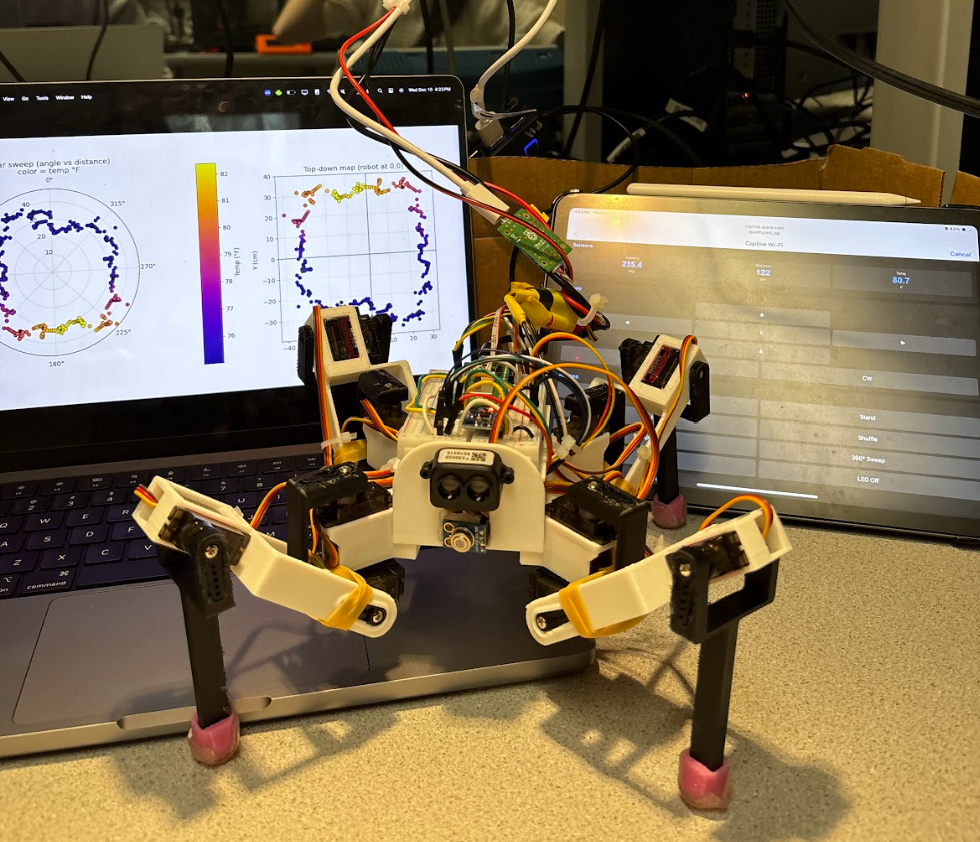
Figure 1: Fully assembled quadruped robot
Summary
We designed and built a 12 degree-of-freedom (3 servos per leg × 4 legs) quadruped robot controlled by a Raspberry Pi Pico W, featuring integrated environmental sensing and a wireless WiFi controller. Starting from a custom CAD body and 3D-printed frame, the robot combines mechanical engineering and embedded electrical engineering to create a platform capable of coordinated four-legged locomotion, heading determination, environmental mapping, and target detection. In order to do so, our system leverages several sensors including an IMU, a solid state LiDAR sensor, and a contact-less infrared sensor.
What We Did
Our project implements a fully functional walking robot with the following key features:
Mechanical Design
We created a custom 3D-printed body and leg assemblies optimized for our specific servo operation requirements and sensor placement. After encountering flexibility issues with initial prints due to insufficient infill, we redesigned the frame to provide rigid mounting points for all four legs and the twelve MG90S servos while accommodating the electronics and wiring on the body through implementing a 2-layer mounting system, enclosing all of the servo cables. The design includes TPU grippy feet for improved traction and stability. The leg files are based off an existing online design, but the attachment to the body and the body itself is all custom to allow for mounting of the Raspberry Pi and sensors.
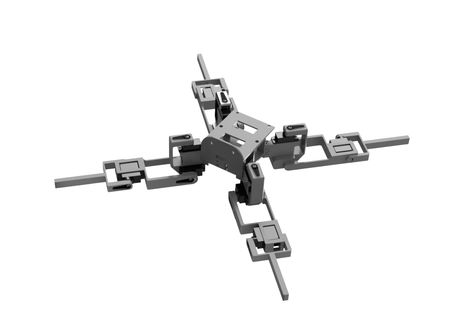
Figure 2: Custom body CAD design
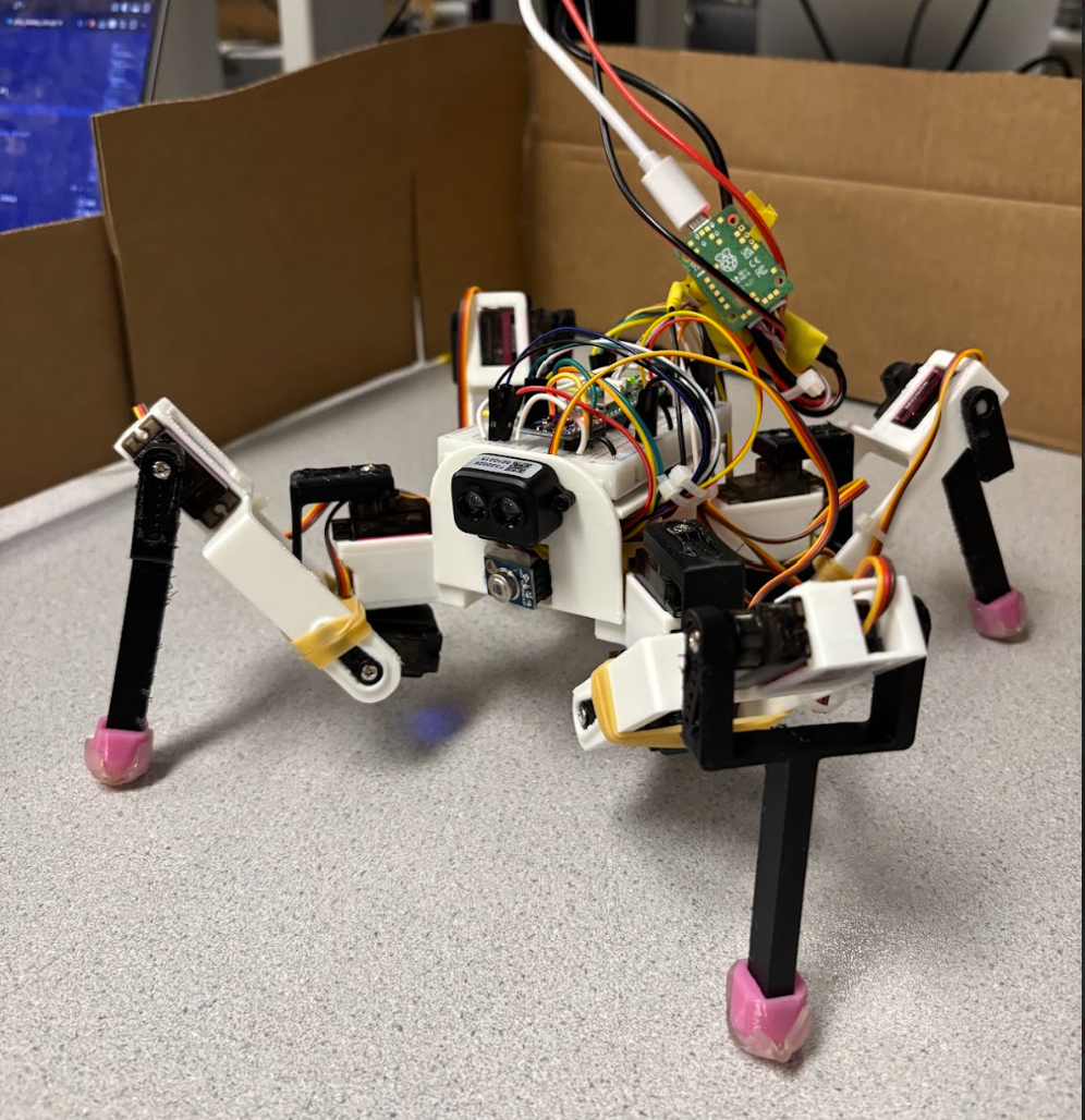
Figure 3: Complete Robot Assembly
Locomotion System
Twelve servos provide three degrees of freedom per leg (joint rotation, thigh angle, and calf angle), controlled via an Adafruit PCA9685 16-channel PWM driver over I2C. We implemented coordinated gait patterns that enable the robot to walk forward, backward, turn in place, and complete fun gestures such as waving, squatting, and shuffling. We took initial servo positions and control sequences for these movements from a Python library (see Appendix) and adapted them for C.
Sensor Integration
The robot features numerous sensors that work together to allow for autonomous navigation and environmental mapping:
- MPU6050 IMU for heading determination and orientation tracking to map the environment
- TF-Luna LiDAR for distance ranging (0.2-8m) to detect obstacles and map surroundings
- MLX90614 infrared temperature sensor for heat signature detection and thermal mapping (effective range ~30 cm for human-sized targets)
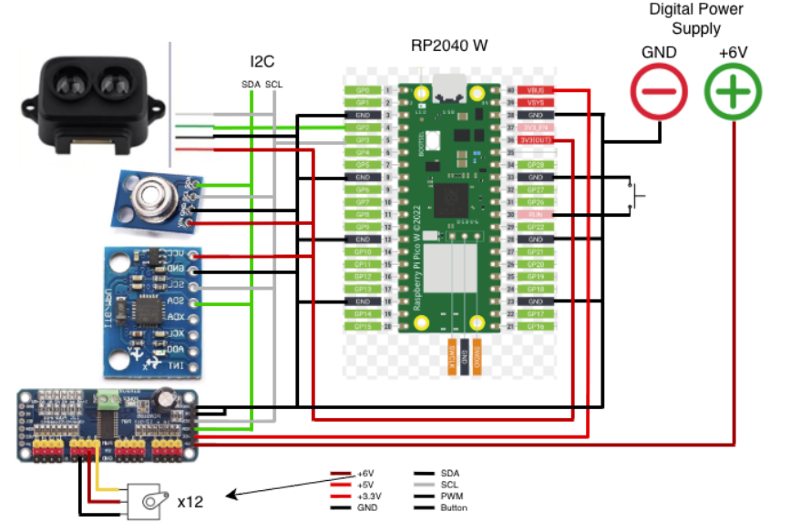
Figure 4: Complete system wiring diagram
Wireless Control
A WiFi-based control interface allows real-time command and control from a computer or mobile device on the local network (we used an iPad), enabling remote operation and monitoring of the robot's sensor data.
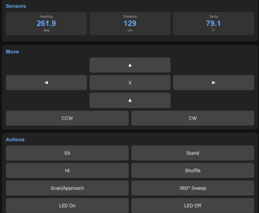
Figure 5: Wifi Controller Interface
Why We Built This
We wanted to create a robot that truly interacts with the world around it. Rather than building a machine that simply responds to pre-programmed commands, we set out to design a sensing platform that could perceive, understand, and navigate complex environments autonomously while moving in a unique and challenging way. The platform we built has the potential to execute various autonomous missions with different sensor-driven objectives.
Inspired by how living creatures use multiple sensory inputs simultaneously, we aimed to replicate this approach of combining data types to make decisions in a robotic platform, and have it sense in ways humans can't, in this case, thermal detection. By combining LiDAR for spatial mapping, infrared sensing for thermal detection, and IMU data for orientation tracking, our quadruped builds an understanding of its surroundings and makes intelligent decisions about movement and target identification.
This project represents the intersection of our mechanical and electrical engineering backgrounds. Coordinating twelve servos in real-time while processing sensor data and maintaining wireless communication pushed us to deeply understand the integration between hardware design, software architecture, and control systems. We chose a quadruped specifically because legged locomotion is more complex than wheeled robots and presents unique challenges in stability, gait coordination, and terrain adaptability.
The practical applications are compelling: quadruped robots with environmental sensing have real-world potential in search and rescue operations (thermal sensing to locate people), industrial inspection in hazardous environments, and exploration of inaccessible terrain. Or even simpler, it can act as a pet and follow you around! Building from scratch gave us the flexibility to customize the sensor suite and control functions for these use cases while demonstrating that sophisticated autonomous robotics is achievable on an affordable microcontroller platform.
High Level Design
Rationale and Sources of Project Idea
Our project was inspired by existing quadruped robot platforms and open-source designs available online. We began by researching quadruped locomotion and found several reference designs on platforms like Instructables and GitHub that demonstrated the feasibility of servo-based legged robots.
Key inspirations included:
- Mechanical Design Foundation: We adapted leg geometry from an open-source 3D-printed quadruped design that provided a proven kinematic structure for three-DOF legs. However, we completely redesigned the body and mounting system to accommodate our specific sensor suite and electronics layout.
- Locomotion Control: Initial servo position sequences and gait patterns were adapted from a Python-based quadruped control library. We translated these movements into C and modified them for our specific servo channel mapping and timing requirements on the Pico W.
- Sensor Integration Approach: The decision to combine multiple sensor modalities (LiDAR, IR temperature, IMU) was driven by our goal to create a robot with perception capabilities beyond human senses. This multi-sensory approach mirrors research in autonomous mobile robotics where sensor fusion improves environmental understanding.
- Platform Selection: We chose the Raspberry Pi Pico W for its balance of computational capability, built-in WiFi, and I2C support, all at a low cost point that makes the project accessible.
The core innovation in our project is not the individual components, but rather the integration of environmental mapping capabilities with legged locomotion on a resource-constrained embedded platform, creating an affordable autonomous sensing robot.
Background Math
Servo PWM Control
The MG90S servos are controlled via PWM signals from the PCA9685 controller. Standard hobby servo control operates at 50 Hz (20ms period). The pulse width determines the servo angle:
- 1ms pulse → 0°
- 1.5ms pulse → 90° (neutral)
- 2ms pulse → 180°
The PCA9685 uses 12-bit resolution (4096 steps). To calculate pulse length in counts:
pulse_length = (desired_ms / 20ms) × 4096
For example, 90° with a 1.5ms pulse: (1.5 / 20) × 4096 = 307 counts
Our servo control function maps angles to PWM values:
uint16_t angle_to_pwm(float angle) {
    // Map 0-180° to approximately 150-600 counts (calibrated for MG90S)
    return (uint16_t)(SERVOMIN + (angle / 180.0) * (SERVOMAX - SERVOMIN));
}

void set_servo_angle(uint8_t channel, float angle) {
    uint16_t pwm = angle_to_pwm(angle);
    pca9685_set_pwm(channel, 0, pwm);
}
IMU Heading Calculation
The MPU6050 provides gyroscope data that we use for heading determination. We integrate angular velocity over time to track orientation:
heading(t) = heading(t-1) + ωz × Δt
Where ωz is angular velocity around the z-axis (yaw rate) measured in degrees per second, and Δt is the time interval.
static inline void update_heading_from_gyro(void) {
    uint64_t now = time_us_64();
    float dt = (now - g_last_gyro_time) / 1000000.0f;
    if (dt < 0.002f) return;

    mpu6050_read_raw(acceleration, gyro);
    float gz = fix2float15(gyro[2]);
    gz += g_gyro_bias; // Apply bias compensation

    // Deadband filter to eliminate drift from small noise
    if (fabsf(gz) < 0.2f) gz = 0.0f;

    g_gyro_heading += gz * dt;

    // Keep heading in 0-360° range
    while (g_gyro_heading < 0) g_gyro_heading += 360.0f;
    while (g_gyro_heading >= 360.0f) g_gyro_heading -= 360.0f;

    g_last_gyro_time = now;
}
Drift Compensation: We use bias calibration and deadband filtering. At startup, we measure the gyro bias while stationary over 200 samples (~400ms), then subtract this bias from all subsequent readings. A deadband filter zeros out readings below 0.2°/s to eliminate integration of small noise values.
static void calibrate_gyro_bias(void) {
    const int samples = 200;
    float sum = 0.0f;
    for (int i = 0; i < samples; i++) {
        mpu6050_read_raw(acceleration, gyro);
        sum += fix2float15(gyro[2]);
        sleep_ms(2);
    }
    g_gyro_bias = -(sum / samples); // Negate to compensate
    printf("Gyro Z bias calibrated to %.3f °/s\n", g_gyro_bias);
}
LiDAR Distance Measurement
The TF-Luna uses Time-of-Flight measurement:
distance = (c × Δt) / 2
Where c ≈ 3×10⁸ m/s (speed of light) and Δt is round-trip time. The sensor outputs distance directly via I2C in centimeters (20-800cm range).
We apply median filtering to reduce noise:
static uint16_t read_lidar_filtered(int samples) {
    uint16_t buf[8];
    int count = 0;
    for (int i = 0; i < samples && count < 8; i++) {
        tfluna_data_t data;
        if (tfluna_read_data(&lidar_sensor, &data) && data.valid && data.distance > 0) {
            buf[count++] = data.distance;
        }
        sleep_ms(2);
    }
    if (count == 0) return 0;
    return median_u16(buf, count); // Returns middle value after sorting
}
Environmental Mapping in Polar Coordinates
For environmental mapping, we store data directly in polar coordinates. Each sample contains:
- θ (theta): Heading angle in degrees (0-360°) from the IMU
- r (radius): Distance in centimeters from LiDAR
- T (temperature): Object temperature in °C from IR sensor
This polar format is ideal for a robot rotating in place, as it directly maps to the robot's heading and sensor readings without requiring coordinate transformation during data collection.
typedef struct {
    float angles[MAX_MAP_SAMPLES];      // Heading in degrees
    uint16_t distances[MAX_MAP_SAMPLES]; // Distance in cm
    float temps[MAX_MAP_SAMPLES];        // Temperature in °C
    uint16_t count;                      // Number of samples
    bool active;                         // Sweep in progress
} env_map_t;
During a 360-degree sweep, samples are collected at approximately 100 Hz. As the robot rotates, each sample is stored with its current heading from the gyro integration, the distance reading from the LiDAR, and the temperature from the IR sensor. The data remains in polar form and is exported to CSV for visualization.
Polar Visualization
Our Python visualization plots the 360° sweep directly in polar coordinates using matplotlib’s polar projection. Angle measurements received from the robot (in degrees) are converted to radians for compatibility with matplotlib:
# Convert angles to radians for matplotlib polar plot
theta_rad = [math.radians(a) for a in angles]

# Create polar scatter plot
ax.scatter(theta_rad, distances, c=temps, cmap="plasma")
Point color represents measured temperature, allowing spatial temperature variation to be visualized alongside distance data.
We also generate a top-down Cartesian map by converting polar coordinates into a robot-centered reference frame:
x = r × sin(θ) y = −r × cos(θ)
# Convert polar to Cartesian for top-down view
x_coords = [r * math.sin(t) for r, t in zip(distances, theta_rad)]
y_coords = [-r * math.cos(t) for r, t in zip(distances, theta_rad)]
This coordinate convention places 0° directly in front of the robot and produces an intuitive top-down environmental map.
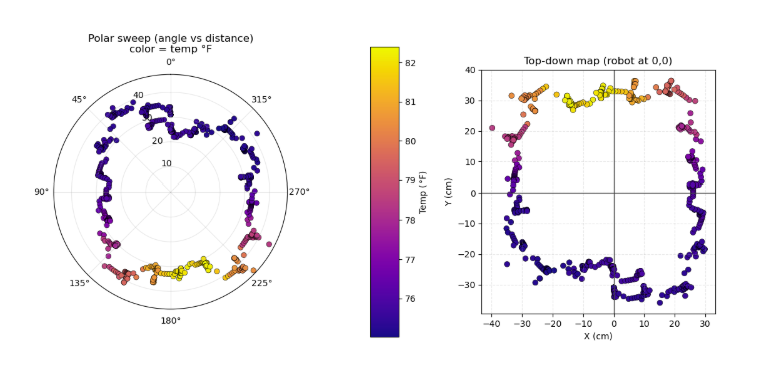
Figure 6: Environmental Map from Robot Sensor Data
Power Calculations
Peak current draw calculation:
Itotal = IPico + (12 × Iservo) + Isensors
Itotal = 200mA + (12 × 250mA) + 160mA = 3.36A
We used a 5V bench supply with 2.5A maximum. Average current during typical operation was ~2A, with gaits naturally staggering servo movements to avoid simultaneous peak loads. Further explanation of the choice to use bench power and the current limitations is discussed in detail in the Hardware/Software Tradeoffs section below.
Average power during typical operation: P = V × I = 5V × 2A ≈ 10W
Logical Structure
Our software follows a modular architecture with clear separation of concerns across multiple files. The codebase is organized into functional groups for maintainability and reusability:
Core Program Files
main.c                    - Main control loop
movement_library.c/.h     - Locomotion primitives
movementlibrary.py        - Python reference
Sensor Driver Modules
pca9685.c/.h             - Servo driver
mpu6050.c/.h             - IMU interface
tfluna_i2c.c/.h          - LiDAR interface
mlx90614.c/.h            - IR temp interface
mlx90614Config.h         - Temp config
Data Structures
mapping.c/.h             - Mapping structures
sensor_data.h            - Global sensor data
Network & Communication
wifi.c/.h                - WiFi AP & web server
dhcpserver/              - DHCP implementation
dnsserver/               - DNS implementation
lwipopts.h               - TCP/IP options
Build & Configuration
CMakeLists.txt           - Build configuration
pico_sdk_import.cmake    - SDK integration
BUILD_WSL.md             - Build instructions
README.md                - Documentation
Data Output
sweep.csv                - Mapping data export
plot_sweep.py            - Visualization script
plot_sweep_csv.py        - CSV plotting utility
Main Control Loop Architecture
The main program coordinates all subsystems through distinct initialization and runtime phases. This architecture ensures that all sensors, communication systems, and movement capabilities are properly initialized before entering the main operational loop.
├── I2C bus setup (I2C1 on GPIO 2/3)
├── I2C device scanning and detection
├── PCA9685 servo driver initialization (0x40)
├── Sensor initialization
│   ├── TF-Luna LiDAR (0x10) - if detected
│   ├── MLX90614 IR temp (0x5A) - if detected
│   └── MPU6050 IMU (0x68) - if detected
├── WiFi access point startup
├── Mapping system initialization
└── Initial robot posture (stand_up, hi, xposition)
Main Loop:
├── Serial Command Processing
│   ├── Movement commands (W/A/S/D/Q/E)
│   ├── Sensor read commands (R, Y, Z)
│   ├── Special actions (H=hi, C=shuffle, B=squats)
│   └── Mapping sweep trigger (N)
├── Background Tasks (continuous)
│   ├── update_heading_from_gyro() - IMU integration
│   ├── refresh_sensor_data() - Sensor polling (~100ms)
│   └── sweep_collect_sample_if_due() - Map data collection
├── Mode Handling
│   ├── ROBOT_MODE_WIFI_CONTROL (default)
│   └── ROBOT_MODE_SCAN_APPROACH (autonomous)
├── Mapping Sweep State Machine
│   ├── Track rotation progress (0° → 360°)
│   ├── Trigger CCW rotation every 2 seconds
│   └── Export CSV when complete
└── WiFi background processing
The modular structure allows individual components to be tested and debugged independently, while the global sensor data structure provides a single source of truth accessible by all modules. The cooperative multitasking mechanism ensures that critical background tasks (heading integration, sensor polling, WiFi servicing) continue executing even during blocking movement sequences by breaking long delays into 10ms chunks with task execution between each chunk.
Hardware/Software Tradeoffs
Onboard vs. Offboard Processing for Map Visualization
Decision: Basic sensor fusion and data collection happen onboard; visualization happens offboard via Python scripts.
Rationale: The Pico has limited RAM (264KB) and no GPU, making real-time graphical rendering impractical. However, the robot needs onboard data storage for autonomous decision-making. By storing data in compact polar format and exporting to CSV, we collect maximum samples while keeping memory usage minimal. We initially tried live WiFi plotting, but this repeatedly crashed due to high data rates. Offboard visualization proved more reliable while retaining autonomous capabilities.
Tethered vs. Battery Power
Decision: Tethered 5V bench power supply (2.5A maximum).
Advantages: Unlimited runtime for extended testing and mapping sessions, consistent voltage regardless of load, no heavy battery weight affecting balance and gait stability, lower total build cost (~$111 vs. $150+ with suitable battery and charging system), no charging downtime between test sessions.
Disadvantages: Cable restricts range to ~2-3 meters and can interfere with motion during turns, power supply current limit (2.5A) below theoretical peak draw (3.36A) means risk of brownouts during simultaneous servo movements, tether creates dependency on nearby wall outlet limiting deployment scenarios.
Mitigation and Reality: Gait patterns naturally stagger servo movements - during a trot gait, only 6 servos (diagonal pair) move simultaneously under heavy load, keeping typical current around 2A average. Simple movements like forward, backward, and gentle turns stay well within the 2.5A limit. However, complex movements like "shuffle" that activate many servos simultaneously did occasionally trigger the overload indicator on our bench supply, causing brief voltage dips. For this educational project, tethered operation was acceptable as our test area was controlled and we prioritized unlimited runtime for iterative testing over mobility. A production version would require a 3S LiPo battery (11.1V, 2200mAh minimum) with a 5V buck converter rated for 4A continuous.
WiFi vs. Bluetooth
Decision: WiFi access point mode.
Rationale: Higher bandwidth supports streaming all sensor data simultaneously (heading, distance, temperature at 10 Hz). Serves full web interface accessible from any browser without custom app development or installation. WiFi power consumption (~50-70mA extra) is negligible compared to servo draw (2000mA average). Longer range (~30m vs. ~10m for BLE) better for outdoor testing. AP mode creates captive portal effect - when iOS/Android devices connect, they automatically open the control page without requiring manual URL entry.
Sensor Fusion Approach
Decision: Simple gyro integration with automatic bias calibration and 0.2°/s deadband filtering.
Rationale: For slow rotation during mapping sweeps (180°/min, 3°/s angular velocity), simple integration with drift mitigation is sufficient. Our testing showed accumulated drift of only 5-10° over full 360° sweep (~2 minutes). Kalman filtering would require accelerometer fusion, add ~2KB code, consume 5-10% CPU, and provide minimal accuracy improvement for this use case. The bias calibration (200 samples at startup) and deadband (0.2°/s threshold) effectively eliminate drift over mapping timescales. For applications requiring absolute heading over hours, a magnetometer would be necessary, but for our 2-4 minute mapping sweeps, gyro-only tracking proved adequate.
Patents, Copyrights, and Trademarks
This project uses open-source components with proper attribution: quadruped leg geometry from Instructables (Creative Commons license), Python movement library reference (MIT License), and Raspberry Pi Pico SDK (BSD-3-Clause). Sensor drivers were developed using manufacturer datasheets and public I2C specifications.
Commercial products (Raspberry Pi Pico W, PCA9685, MPU6050, TF-Luna, MLX90614, MG90S servos) are trademarks of their respective manufacturers and were used as intended. Our original contributions include the custom body CAD design, C-based movement library adaptation, environmental mapping algorithm, WiFi control interface, gyro drift mitigation, autonomous sweep state machine, and visualization scripts.
While quadruped locomotion and sensor fusion are extensively patented by companies like Boston Dynamics, our educational implementation uses different mechanisms (hobby servos vs. electric/hydraulic actuators), operates at smaller scale (30cm vs. 1m+ body length), and employs publicly known techniques (PWM control, I2C communication, gyro integration). As an educational project for ECE 4760 at Cornell University, we properly cite all external resources, and the integration work and software architecture represent our original engineering effort. No NDAs were required as all components were purchased through standard retail channels with publicly available documentation.
Program/Hardware Design
Overview
Given the ambitious nature of our project, a primary component of our software implementation is properly combining several embedded sensors so that our main processor (RP2040) can respond to the environment and relay information with our WiFi controller. The sensors used in our design, in the order in which they were implemented, are as follows: servo driver, WiFi access point, LiDAR distance sensor, infrared thermometer, and inertial measurement unit (IMU). Our software leverages standard I2C communication and high processing speed to read and update environmental variables. A modular organization includes several libraries dedicated to each peripheral for simplified execution in our main file where initialization, control, and scheduling take place.
The primary difficulty regarding software revolved around successfully implementing our WiFi access point. At first we had mistakenly implemented Bluetooth control, but quickly realized that this was beyond the usable scope of our wireless controller as we had envisioned (Bluetooth would be better suited for inter-Raspberry Pi communication). We followed Bruce Land's source code and were quickly able to get the example LED code running, but adding any new complexity to the page itself quickly crashed our interface, producing our error page repeatedly. With minimal debugging capability, this proved to be the greatest difficulty, though it was eventually achieved.
Figure 7: Complete system wiring diagram
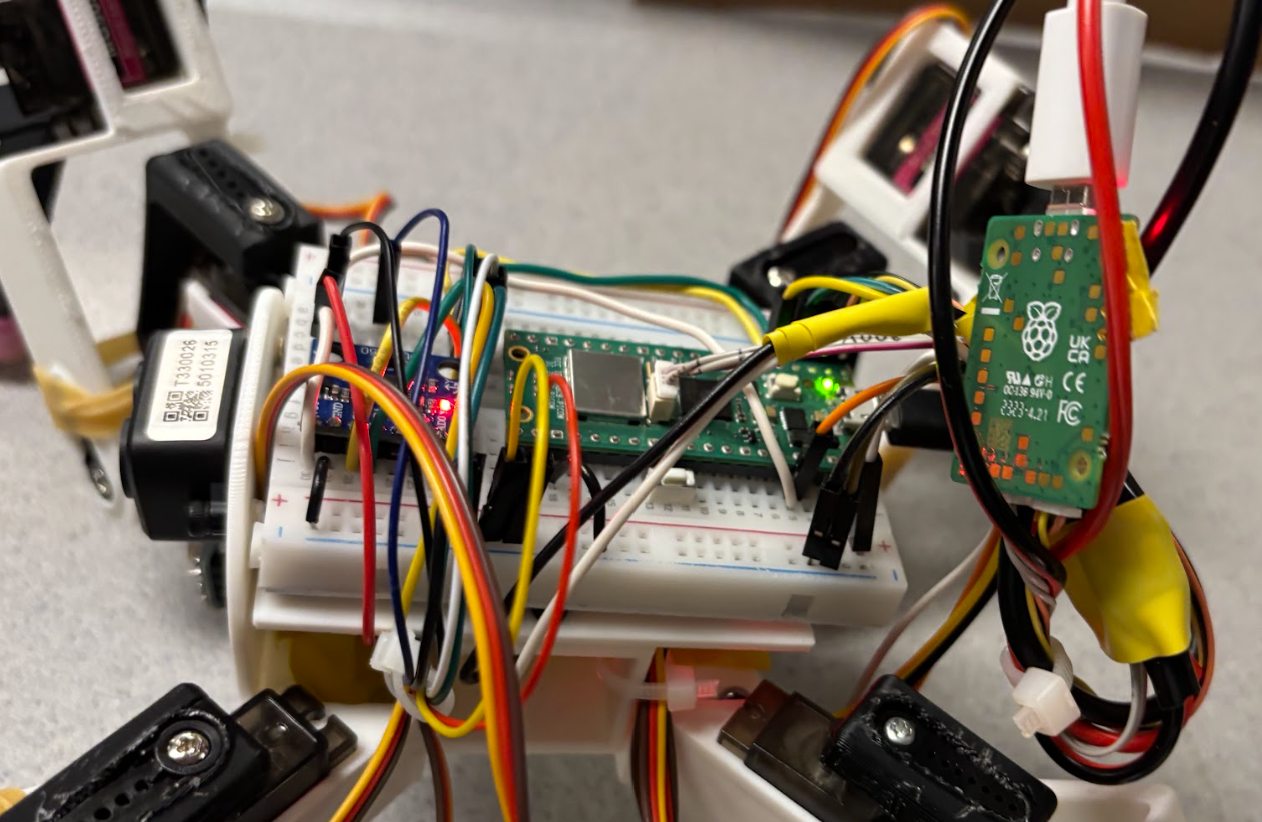
Figure 8: Complete system wiring on the Robot
Servo Driver
Our servo driver provides low-level servo control through hardcoded poses composed of individual servo assignments. The RP2040 communicates with a 16-channel PWM IC (PCA9685) over I2C to offload PWM generation to dedicated hardware, simplifying port management by freeing up PWM pins and simplifying timing constraints since the Raspberry Pi Pico is primarily occupied with WiFi updates, sensor reads, and program control.
On startup, the PCA9685 is initialized by storing both the I2C instance and its address before preparing each servo. The included library encapsulates this into a single pca9685_init() function which we use to start our program and thereafter set all 12 servos to a known initial pose: a combination of both "standing" and "X-position". Another library function called pca9685_set_pwm_freq() converts our desired PWM frequency (60 Hz) into a prescaled register value. This pairs with our primary function pca9685_set_pwm() to write 12-bit on and off pulses to each channel register in order to set channel pulse width and thus change each servo's position.
Positioned one logical level above this, our movement_library.c handles the translation of individual poses called in main.c to individual servo positions. Poses and actions such as forward(), cw(), stand(), and right() are all composed of hardcoded joint configurations. To eliminate some additional abstraction, servo channels are translated into named entities that each have their own PWM controller functions. Thus, forward() contains sequenced joint movements. Each of these functions undergoes an angle-to-PWM conversion angles_to_pwm() as previously described in the Background Math section.
// Movement function example
void forward(void) {
    calf_4(45);
    calf_1(45);
    thigh_1(160);
    thigh_3(160);
    joint_1(100);
    joint_3(90);
    coop_sleep_ms(100);
    joint_2(160);
    joint_4(60);
    coop_sleep_ms(200);
    thigh_2(135);
    thigh_4(135);
    // ... continues
}
In order to maintain sensor communication during robot movement, a cooperative background function is utilized in replacement of sleep_ms(). Specifically, coop_sleep_ms() maintains timing control while preventing background starvation for all of the I2C sensors. As opposed to blocking execution for the full delay time, this function loops through a predefined MOVEMENT_SLEEP_STEP_MS, executing a background sensor read and refresh after each step until the full delay has been accounted for. This background routine called robot_background_tick() exists in our main.c file and updates sensor and control values for live continuous operation. This separation is critical for mapping data collection, accurate heading, and WiFi access page servicing. By using a predefined sleep step, we are able to accurately configure timing constraints across movement and real-time programs.
WiFi Access Point
Wireless communication is implemented using the Pico W and lwIP networking stack, following Bruce Land's WiFi access point (AP) example code. Our system produces a well-defined AP with live sensor data and several buttons to control both the robot's motions as well as its programmable scripts. The AP allows for direct local connectivity without additional infrastructure, supporting predictable latency characteristics.
The Pico W's initialization library starts up the on-chip CYW43 driver which configures the WiFi credentials and launches the networking stack including DHCP and DNS services. A TCP server handler manages incoming connections, prompting communication between the robot and the client controller. Sensor data such as heading, distance, and temperature are all transmitted to the controller at 10Hz. On the other side, over 15 buttons control robot movements and actions.
Figure 9: Wifi Controller Interface
The webpage itself is implemented directly as an HTTP server using TCP callbacks, in which each GET request is parsed and organized to a given endpoint such as /sensors, /cmd, and /map. The sensor endpoint features validity flags for each printed value so that in the case of disconnected sensors the controller will read "--" for missing values. If the lwIP send-buffer is not available before sending large messages, the transmission will not be executed in order to prevent data loss or corruption.
A fun and very useful feature is our test_server_content() function which detects iOS connections through their "/hotspot-detect.html" request in order to automatically open the main controller page. Similar functions exist for both Android and Windows users though they were not utilized in our implementation.
Network servicing is also implemented cooperatively using a background refresh function in order to prevent processing backlog and delays. Both motion and action functions are executed outside the TCP receive handler. This means that button presses on the controller load commands on the Pico W into a fixed buffer which is dequeued and executed by wifi_ap_background(). This design prevents blocking functions from delaying the access point's responsiveness.
LiDAR Distance Sensor
Our LiDAR distance sensor is implemented using a TF-Luna sensor with I2C communication across three layers of abstraction: reading raw data, filtering measurements, and publishing to the global sensor structure.
In order to read raw sensor data, tfluna_read_data() executes I2C register reads and returns both distance and a matching validity field. We then filter these results using read_lidar_filtered() to conduct several measurements in a loop. These measurements are added to a buffer if their data is valid. This buffer's median is then read as the real distance value. The median was chosen to neglect interference from incorrect boundary readings (0 and values >>100 cm). If no data is valid, the function returns a failing value of 0. This filtered distance is then integrated into the whole system by the update_sensor_data() and refresh_sensor_data() functions. These update the global sensor data structure consisting of both measurement and validity flags. A global data structure was necessary to allow data to be both written in main.c and read in wifi.c. LiDAR refresh occurs at approximately 10 Hz to take full utilization of the I2C bandwidth and provide useful telemetry.
The LiDAR data itself is used primarily in the quadruped's mapping function, but is also printed to the WiFi controller interface. In wifi.c, the /sensors endpoint transmits this filtered data for display. For mapping, distance values are sampled at an even higher frequency during active sweeps (~100 Hz) to be stored alongside heading and temperature to create the environmental map.
Infrared Temperature Sensor
We interface with the MLX90614 non-contact infrared thermometer over I2C to read surrounding objects' temperatures at a distance. Similar to the LiDAR, several layers of abstraction exist to read register data, filter the measurements, and publish the data. An existing Arduino library for the MLX90614 was translated to C for our use case. The device can be found at its default address 0x5A.
Our mlx90614.c library reads temperature values by conducting two-byte reads from the sensor's registers. Each temperature register consists of 16 bits with 15 of those bits containing data. The two important registers we interface with are 0x07 (object temperature) and 0x06 (ambient temperature). A function mlx90614_read_both_temps() reads from both of these registers and creates 32-bit floating-point values using the following logic:
Temp(K) = raw_value × 0.02
Temp(°C) = Temp(K) − 273.15
This data is then filtered using a read_temp_filtered() function which calls the read routine and sums all successful samples in the provided size parameter. Calculating the mean produces an appropriately filtered measurement given that temperature can only slowly vary.
As was the case before, filtered measurements are updated to the global sensor data structure for both WiFi and mapping purposes. In order to provide more meaningful data to those who use the imperial system, we also translate this data from Celsius to Fahrenheit before printing it to the user. A validity flag is also utilized to ensure that the data is only interpreted when it is accurate and updated.
Inertial Measurement Unit (IMU)
Communication with our inertial measurement unit (MPU6050) also occurs over I2C at the default address 0x68. Our code integrates this three-axis accelerometer and gyroscope to generate accurate heading data. Sensor data about the z-axis is used to determine the rotational velocity from which real-time quadruped heading is derived.
Raw IMU data is read in bursts from the ACCEL_XOUT_H (0x3B) register, where only the last two bytes are used in our case, corresponding to gyroscope readings in the z-direction. Each of these readings is a signed 16-bit integer which mpu6050_read_raw() turns into int16_t arrays. These measurements are then converted to floating point using fixed-point scaling before converting from angular rate to degrees per second.
During testing, we discovered that our gyroscope experienced constant drift. In order to fix this issue, we added bias calibration through calibrate_gyro_bias() which gets 200 measurements while the robot is stationary, converts each sample to floating point, computes the mean, and then stores this value as the global bias term. This was certainly a creative solution to a frustrating problem. However, this produced errors between different implementations of our code and was eventually scrapped for a default bias which is predefined in our codebase: GYRO_Z_BIAS_DEFAULT. The value we found sufficient was 2.5°/s.
In order to determine heading, we implemented update_heading_from_gyro(). This function first saves the current time in order to track the elapsed time, then integrates the gyro reading over the time interval. The heading variable is saved as a 32-bit float in degrees and kept within the 0-360° range.
The last data handling step is filtering, where we take this integrated heading and push it through a low-pass filter. This filter, implemented in our smooth_heading() function, finds the smallest angular difference between updates and applies exponential smoothing (α ≈ 0.15) for optimal filtering. The idea of exponential smoothing was actually an AI recommendation that proved useful. The filtered heading is then saved to the global sensor data structure for proper program handling.
Main Control Program
The primary level of our programming design exists in our main.c file where global state is managed through a cooperative loop that combines motion commands, sensor collection, WiFi servicing, and both mapping and scanning execution. The file consists of initialization and event loop, global state logic, sensor processing functions, and behavior routines.
Main.c exists at the top level above all of its supporting libraries, which is why it includes a lengthy list of supplementary C files as previously described in this section (a .h file for each sensor and more). I2C is configured to 100kHz and SDA and SCL are declared on the RP2040's GPIO 2 and 3 and are pulled up to active high logic as necessary. At startup, i2c_read_timeout_us() is used to scan expected I2C addresses and alert whether an ACK has been received back from the address as opposed to a NACK or timeout. Flags for each sensor are then set high for active and remain low if detection fails (Flags: g_found_lidar, g_found_imu, g_found_temp, and PCA9685 driver). If flags are high for the given sensor/driver, the respective init() is called to start up the system. Given elaborate difficulties with getting our first temperature sensor to communicate over I2C, we implemented further logic to secure communication. If the initial detection fails, a dedicated routine will attempt to read and check the dedicated temperature register address. All sensor outputs from active sensors are published to the global structure so that local logic and the WiFi server can use real-time values.
Several helper functions exist to sample and filter the raw data from the sensors:
median_u16()takes the fixed buffer from the LiDAR and performs the median operator to filter distance measurementsread_lidar_filtered(int samples)collects several successful measurements and returns the result usingmedian_u16()read_temp_filtered(int samples)takes several measurements and returns the average of successful samplessmooth_heading(float raw_deg)applies exponential smoothing to reduce jitter at both boundaries (0° and 360°), finds the shortest angle delta within ±180°, updates filter state, and clips the result to [0,360]
A neat feature of our main file is that you can directly control the quadruped over serial. Upon startup, our program prints the menu of controls which includes the complete list of movement and action capabilities. Entering the respective character into the serial terminal will trigger getchar_timeout_us() which prints back a fun response and then activates the expected result. For example, entering "P" or "p" into the serial terminal and pressing enter will print back "Ending Program\n", call legs_up() from the movement library (which looks like a dying spider), and then print "Please! I don't want to go\n" before ending the program.
An important attribute we wanted to add to our robot was an aspect of autonomy. Thus, we designed two scripts that could be run fully autonomously to produce meaningful results or interactions. The first is an environmental mapping script.
Environmental Mapping Script
The mapping script is implemented using a coordinated 360-degree sweep that samples heading, distance, and object temperature over time and stores the results in a fixed buffer for CSV export and offline visualization. A global data structure for mapping consists of arrays for angles[], distances[], and temps[], in addition to a data count field and an active flag (g_map). This script only runs when either the WiFi controller selects the "360° Sweep" button or the mapping character is called in the serial terminal. At which point the g_map flag is set high and the function will be triggered in our main loop.
In wifi.c, the button request is parsed in test_server_content() and triggers start_mapping_sweep() to initialize the sweep data and enable sensor collection. Data sampling is performed by sweep_collect_sample_if_due() using the previously discussed cooperative background refresh. This function is specifically rate limited at 100Hz to provide enough data points for efficient and productive mapping results. When measuring heading, this function will use the global heading reading when it has a valid flag, but will otherwise rely on the unfiltered integrated heading to provide continuity in extreme environments. This heading is also passed through smooth_heading() to provide safe wraparound conditions and reduce noise/jitter. Distance is then obtained through read_lidar_filtered(5) and temperature through read_temp_filtered(2). In order to exclude errors and noise, if any sensor returns -1 the data point is neglected. Similarly, if the distance is greater than 100 cm we choose to neglect the data (though this is configurable) so as to produce a more localized map even in a large room.
Successful samples are added to the map buffer with map_add(&g_map, heading, dist, temp). This adds angular normalization to heading and adds a new entry or merges with an existing entry when the new heading is close to a previously stored heading within a set angular tolerance. Merging reduces redundancy which can occur during stale or slow movements. Live data points are printed to the serial terminal enabling real-time debugging and observation.
The sweep rotation is managed in the main loop as a simple iterable state machine which rotates using cw() or ccw() depending on the configuration. Sampling runs concurrently in the background during all movements, active and passive. Rotation ends when the accumulated heading has achieved at least 360 degrees. Once met, the g_map flag is set low and data is exported into CSV format using dump_map_csv(). Each point consists of [angle_deg, distance_cm, temp_c]. This function dumps all recorded data points (2000 maximum) into the serial terminal for quick copy and pasting.
An offline Python script can then be run on the produced CSV file to visualize the mapping results on your primary computer. Both a polar and Cartesian coordinate graph are generated with point color representing object temperature.
Our Python script, plot_sweep_csv.py, parses through each line of the provided CSV using Python's csv.reader to split rows by commas and then records angle, distance, and temperature into float lists after filtering out invalid or incomplete rows. In this manner, it rejects the header row (entry 0). Given that the robot remains at heading 0 for a long period of time during the start of our mapping script, these entries are neglected for easier visualization.
A helper function plot_sweep(ang, dist, temp) implements the remaining plotting logic. Temperature is converted from Celsius to Fahrenheit as previously described, and the color scale plot is normalized to the minimum and maximum of the dataset using Normalize(vmin, vmax). Angles are converted to radians using math.radians since Matplotlib polar axes use radians not degrees. Then, Cartesian coordinates are generated using the standard polar-to-Cartesian transformations:
x = r × cos(θ)
y = r × sin(θ)
The actual visualization uses Matplotlib to place three different figures: a polar scatter plot on the left, a Cartesian scatter plot on the right, and a vertical color scale in between. In the polar plot (ax_polar), the script calls scatter(theta, distances, c=temps_f, cmap=cm.plasma, norm=norm, ...) so that each sample is created as desired. Its axis is configured with set_theta_zero_location("N") so 0 degrees occurs at the very top of the plot, and set_theta_direction(1) so angles increase counterclockwise (consistent with our real sweep). In the Cartesian plot (ax_cart), the script scatters (x, y) with the same colormap and normalization so the two plots share the same temperature relationship. This draws axes lines at x=0 and y=0 to mark the robot's starting point, and measurements are in cm.
Figure 9: Environmental Map from Robot Sensor Data
On program completion, the Python script prints the total number of samples and launches the plots with plt.show(), which blocks until the user closes the resulting figure. A difficult step was trying to get our C program to automatically call this Python file and display the results on our WiFi AP, but we were restricted by the size of data that we could pass through our WiFi buffer. Implementing C-to-Python communication from the Raspberry Pi to the primary computer also proved significantly more daunting with difficult serial errors. This was eventually achieved but at very low data transmission rates. Live mapping was executed but was eventually scrapped given its complexity and slower data measurement rate.
Thermal Scanning Script
Our scanning program implements a scripted temperature scan of its forward-facing environment using controlled rotational motion to record the orientation with the highest detected object temperature before approaching this high-temperature object and waving hello. This program is triggered either from the serial command interface or via the WiFi AP with the "Scan/Approach" button.
At the start, the quadruped rotates counterclockwise 4 times, corresponding to roughly a 90-degree rotation depending on the surface friction. Then our robot takes a temperature reading before rotating clockwise for a total of 9 samples, corresponding to roughly a 180-degree sweep from the starting position. After each rotation, the program calls refresh_sensor_data() to update all telemetry data, guaranteeing that the robot's recorded temperature value matches the corresponding heading. Each temperature sample is stored in an array indexed by the current rotation number. The program tracks the largest value and checks whether each new measurement surpasses the previous value, replacing the maximum value if so. The program saves the largest temperature's index in order to recall what orientation the maximum occurred at, and more specifically how many turns it will take to return to this orientation. Upon scan completion, the routine finds the difference between the current number of rotations (8) and the index for the maximum temperature. A while loop depletes the rotations by going counterclockwise until the two are equal.
At this point, the robot begins moving forward(), approaching the hot object. Only once the object is detected using the LiDAR at less than 10 cm away, the robot will halt and say hello using the hi() function. Throughout the entire thermal sweep process, motion commands are blocking, but background servicing remains active through cooperative scheduling.
Mechanical Design
Figure 10: Full CAD Assembly Front View
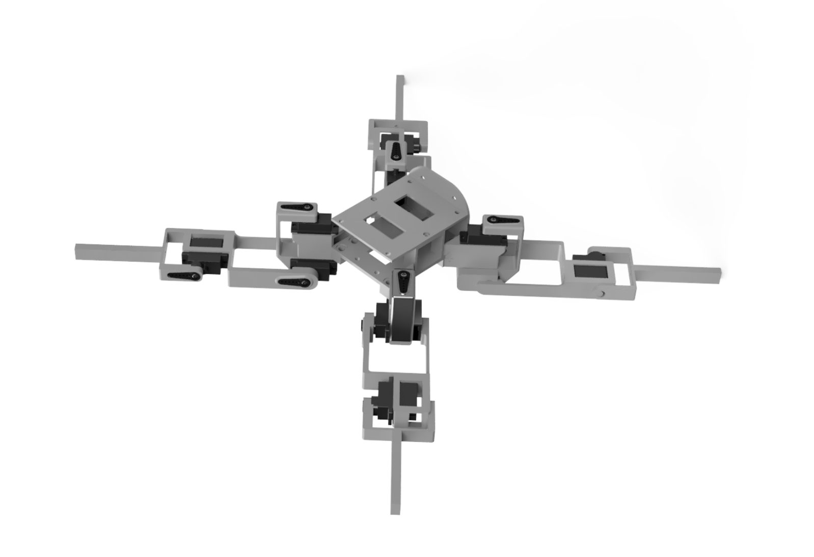
Figure 11: Full CAD Assembly Back View
Custom Body Design
The robot's body is a completely custom design created in CAD to address the specific requirements of our sensor suite and electronics layout. Unlike the legs, which were adapted from an existing open-source design, the body was designed from scratch to provide optimal mounting for the Raspberry Pi Pico W, sensor array, and power distribution system.
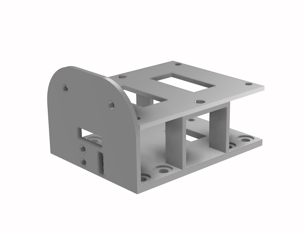
Figure 12: Body CAD Front View
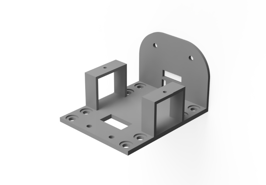
Figure 13: Body CAD Back View, Top Plate Remvoed
Key Design Features:
The body implements a 2-layer mounting system that separates the servo driver and servo wiring (lower layer) from the microcontroller (upper layer) and sensors (front plate). This vertical stacking approach minimizes the robot's footprint while providing organized cable management. All servo cables route through internal channels and are enclosed within the body structure, preventing them from interfering with leg motion or snagging during operation.
Four corner mounting points attach the legs to the body using two M4 heat-set inserts and screws in each position. The body includes cutouts for cable routing for the fore-mounting sensors: LiDAR sensor (forward-facing), IR temperature sensor (forward-facing below the LiDAR), and IMU (centered for accurate heading measurement on the top of the body).
Additional mounting provisions use M2.5 heat-set inserts (14 total) to secure the Raspberry Pi Pico W, PCA9685 servo driver board, and the sensors on the fore plate. The design accommodates all cable routing and bend radii. While the original design intended for a soldered breadboard to be secured with M2.5 screws, we ended up using the sticky backing on the breadboard to secure it to the top of the body, which proved adequate for our needs.
Leg Design and Assembly
The leg design was adapted from an open-source 3D-printed quadruped (see Appendix D for complete source listing). Each leg consists of three segments (joint, thigh, calf) providing three degrees of freedom per leg, for a total of 12 DOF across the robot.
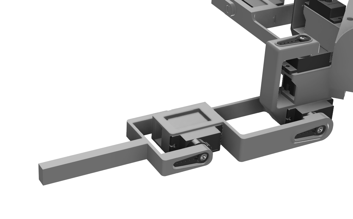
Figure 14: Leg assembly
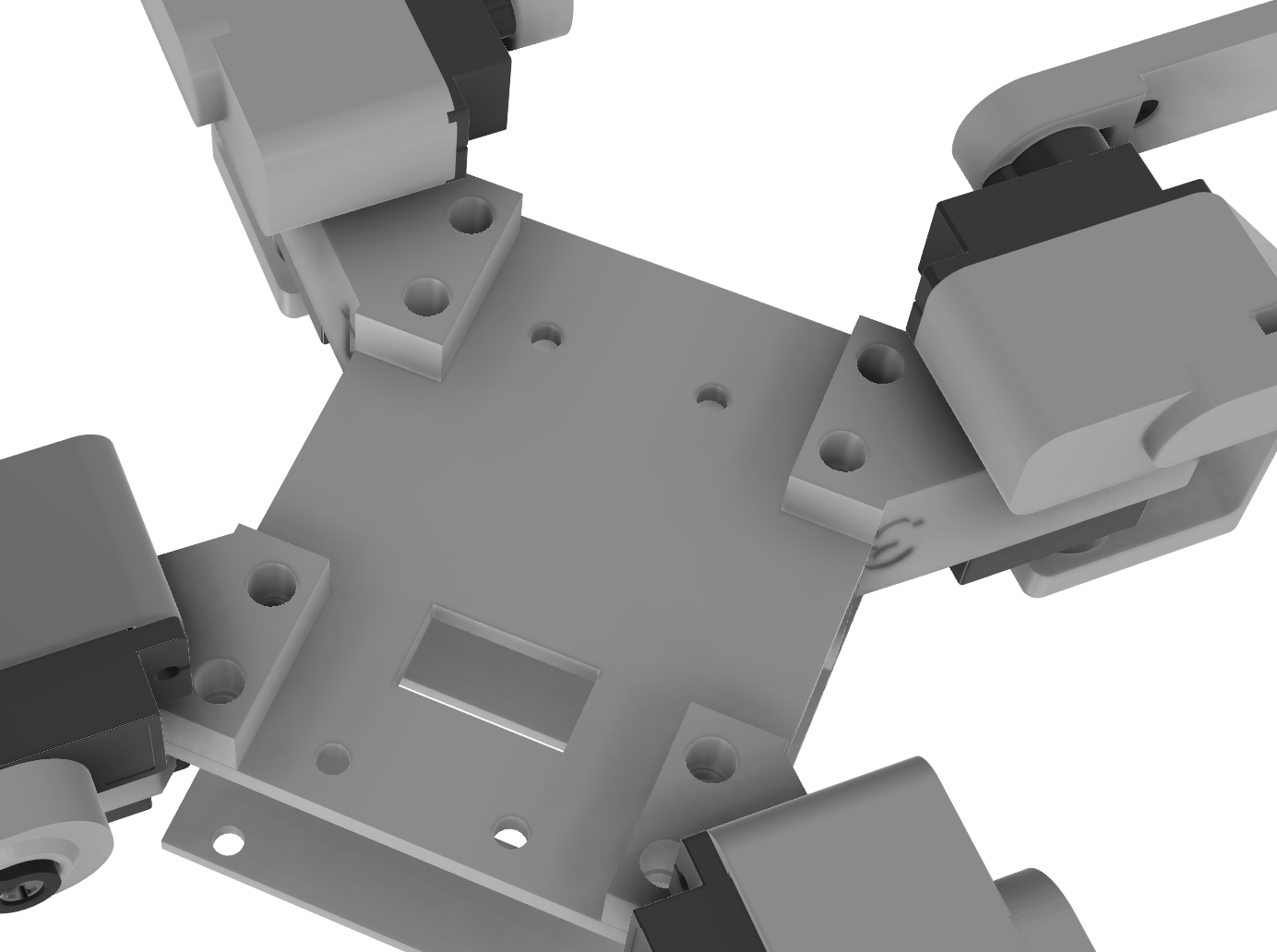
Figure 15: Leg Attachment to Body via M4 Screws & Heat-Set Inserts
Leg Kinematics:
Each leg features:
- Joint servo/hips (rotation): Enables leg rotation around the vertical axis for steering and strafing motions
- Thigh servo (elevation): Controls leg lift height for swing phase during walking
- Calf servo (extension): Adjusts leg reach and ground contact angle
The three-segment design allows for a wide range of motion and enables both simple gaits (alternating diagonal pairs for trot gait) and complex maneuvers (individual leg control for turning in place).
Foot Design:
The original design specified TPU (thermoplastic polyurethane) feet for their flexibility and grip properties. While TPU provided some cushioning, it proved less grippy than expected on smooth surfaces. Gorilla tape was applied to the bottom of each foot to enhance traction, which dramatically improved walking stability and prevented slipping during turns.
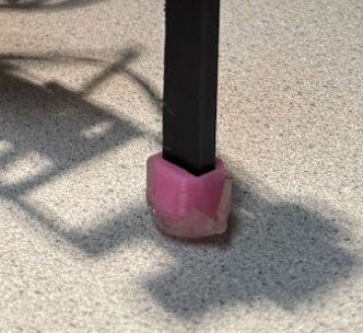
Figure 16: TPU feet with Gorilla tape applied for improved traction
Design Iterations
The initial body print exhibited excessive flexibility due to insufficient infill percentage, causing motion quality issues as the frame flexed under servo loads. The design was revised with increased wall thickness and infill along with thicker dimensions (the base plate is now 3mm), providing the necessary rigidity. The leg attachment points were also reinforced with thicker printing settings. Print settings were optimized for a Bambu X1C printer.
Assembly Method and Considerations
The modular design allows for easy maintenance and component replacement. Leg segments connect to each other through the servo horns and a snap-in bump. The joints/hips connect to the body via M4 heat-set inserts and screws. The joint-to-thigh connection proved looser than desired after 3D printing due to its length. Rubber bands were added as reinforcement to eliminate play in this critical joint, significantly improving motion quality and preventing position drift.
Servos can be removed individually by extracting the M4 screws, and electronics are accessible by removing the upper body layer. Heat-set inserts provide reusable threaded connections that don't degrade with repeated assembly/disassembly cycles, unlike direct threading into plastic. Cable routing was carefully planned to prevent interference with moving parts, with all servo cables running through designated channels in the body and secured with zip ties at strategic points. Power wires are kept separate from signal wires to minimize electrical noise, and all exposed power connections are insulated with electrical tape for safety.
The final assembled robot measures approximately 30cm × 30cm × 5cm (L × W × H) when splayed into the neutral X-position.
Assembly Notes: The servos are positional. When first setting up the legs, you must not attach the servo horns. The setup_servos() command must be uncommented in main and then the servos should be attached to each joint via the servo horns and set screws once that program is running. This ensures that each joint is in the position it thinks it is in.
Bill of Materials
| Component | Description | Quantity | Cost (USD) | Source |
|---|---|---|---|---|
| Electronics | ||||
| Raspberry Pi Pico W | Main microcontroller with WiFi | 1 | $7.00 | Raspberry Pi |
| MG90S Servos | Metal gear micro servos for leg actuation | 12 (16-pack) | $28.99 | Amazon |
| Adafruit PCA9685 | 16-channel 12-bit PWM servo driver | 1 | $14.95 | Adafruit |
| MPU6050 IMU | 6-axis accelerometer and gyroscope | 1 | $9.59 | Amazon |
| MLX90614 | Non-contact infrared temperature sensor | 1 | $11.99 | Amazon |
| TF-Luna LiDAR | Time-of-flight distance sensor (0.2–8 m) | 1 | $23.37 | Amazon |
| 5V Power Supply | Bench power supply (2.5 A) | 1 | N/A | Lab equipment |
| Jumper Wires | Breadboard connections | Assorted | N/A | Lab |
| Mechanical Components | ||||
| PLA Filament | 3D printed body and leg structures | ~200 g | ~$1.00 | Engineering |
| TPU Filament | Flexible feet material | ~50 g | ~$1.00 | Engineering |
| M4 Heat-Set Inserts | Leg mounting hardware | 24 | ~$2.00 | Engineering |
| M4 Screws | Leg assembly fasteners | 24 | ~$3.00 | Engineering |
| M2.5 Heat-Set Inserts | Electronics mounting hardware | 14 | ~$2.00 | Engineering |
| M2.5 Screws | Electronics mounting fasteners | 14 | ~$2.00 | Engineering |
| Zip Ties | Cable management | Assorted | ~$1.00 | Lab |
| Rubber Bands | Joint reinforcement | ~10 | ~$1.00 | Lab |
| Gorilla Tape | Foot traction enhancement | 1 roll | ~$2.00 | Engineering |
| Total Estimated Cost | ~$111 | |||
Things That Didn't Work
- Live mapping visualization on Pico: We tried creating the mapping visualization plot on the Pico and streaming it to the WiFi interface, but it repeatedly crashed the website due to memory constraints and data buffer limitations.
- Temperature sensor integration: The MLX90614 temperature sensor took considerable time to integrate properly. We debugged it by first getting it running in C++ via Arduino since there's an Arduino library for it with plenty of example code online. We used that to ensure the sensor worked, then translated everything to work with the Pico.
- Blown servo driver boards: We (Sarah Grace, oops) blew multiple PCA9685 servo boards by connecting V+ and VCC flipped. This was a costly learning experience about double-checking power connections!
AI Usage
We used AI tools extensively throughout the project for debugging:
- Debugging C code when encountering I2C communication errors and timing issues
- Helping transcribe the original Python movement library to C code, adapting the structure for our servo channel mapping
- Assisting with sensor .c and .h file creation and cross-checking against datasheets to ensure correct register addresses and I2C protocols
- Suggesting the exponential smoothing filter approach for IMU heading, which proved very effective
- Helping troubleshoot WiFi connectivity issues and TCP buffer management
- Helping format our final report into HTML for this website
Results
Test Data and Demonstrations
Environmental Mapping
The mapping system successfully captured detailed environmental profiles combining distance and temperature data. The polar coordinate plots clearly show obstacles detected by the LiDAR and thermal signatures identified by the IR sensor. The square shape of the cardboard barrier enclosure is clearly visible in the resulting map data, demonstrating accurate spatial reconstruction from our sensor fusion approach. We placed hot and cold beverages in each corner of the mapped area to clearly demonstrate the system's thermal detection capabilities and spatial accuracy.
Figure 17: Environmental Map from Robot Sensor Data
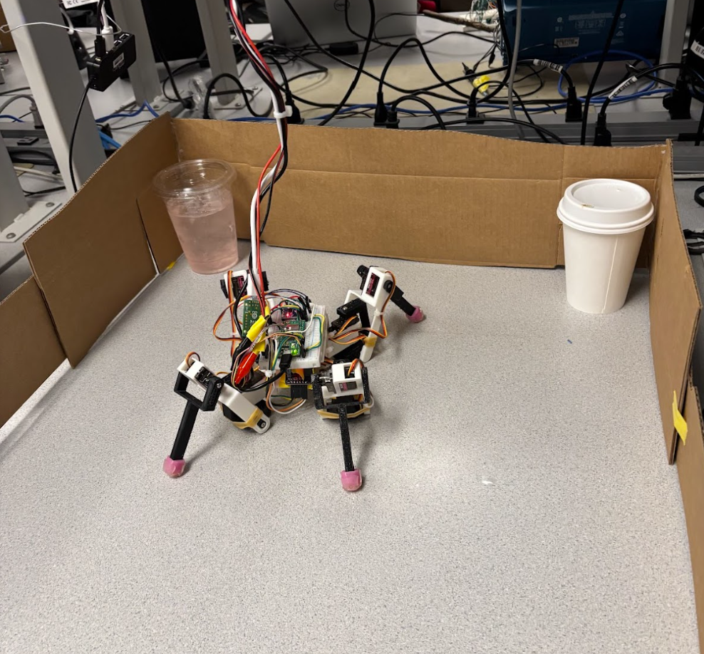
Figure 18: Physical test environment showing cardboard barrier setup and beverage placement
Video demonstrations:
- Autonomous 360° scanning sweep with live data collection
- Thermal target identification and autonomous approach behavior
- WiFi control interface demonstration with real-time telemetry
Video of Temperature Readings:
Scanning Clip:
Speed of Execution and Responsiveness
The robot demonstrated minimal hesitation during operation and worked as expected. Movement commands from the WiFi controller were executed immediately with no perceptible lag. The cooperative multitasking implementation successfully maintained sensor updates during movement sequences without causing motion stuttering or interruption. The 360-degree mapping sweep collected samples at approximately 100 Hz while simultaneously rotating and updating heading calculations, demonstrating effective concurrency on the single-core Pico W. Serial command processing responded instantly to user input. The web interface updated sensor telemetry smoothly without affecting movement control performance.
Accuracy
The gyro integration with bias calibration and deadband filtering demonstrated minimal drift, returning to the starting orientation within 5-10 degrees after a full 360-degree rotation over approximately 2 minutes. The TF-Luna LiDAR achieved repeatability within ±2 cm as specified in the datasheet, with median filtering successfully rejecting noise. The MLX90614 IR thermometer accurately identified warm targets (such as a person's hand) against cooler backgrounds. The sensor's 90° field of view means the effective range depends on target size; for larger objects like human body parts, detection worked reliably at approximately 30cm (1 foot), while smaller objects required closer proximity. All sensor data was easily copied from the serial monitor to CSV format without corruption, and the resulting environmental map clearly shows the square geometry of the cardboard enclosure and placed objects, confirming spatial accuracy.
Safety Design
Safety was enforced through multiple design considerations. All power supply connections were covered in electrical tape to prevent shorting and protect users from exposed conductors. The system operates at 5V, well below electrical shock hazard threshold, with common ground connections preventing voltage differences. The robot has minimal force capability due to small servo size and lightweight construction, making it incapable of causing injury. The TF-Luna uses an eye-safe Class 1 laser, the MLX90614 IR sensor is completely passive, and the MPU6050 is self-contained with no external emissions. The WiFi control interface allows safe-distance operation, and emergency stop is available by unplugging power or pressing 'P' on the serial terminal.
Usability
The robot proved highly usable for both our team and outside users. The WiFi control interface provides intuitive operation as users simply connect to the "quadruped_ap" WiFi network (password: "password") and navigate to the robot's IP address in any web browser. No software installation or configuration is required. The interface presents clearly labeled buttons for all movement commands with real-time sensor readings displayed. We successfully demonstrated the robot to classmates who controlled it immediately without instruction. The serial terminal interface provides advanced functionality for users comfortable with command-line interaction. Setup time is minimal - plug in power, wait for WiFi to initialize (~10 seconds), and connect. The robot's portable form factor and robust construction allowed easy transport between testing locations and graceful recovery from tip-overs during testing.
Figure 19: WiFi Controller Interface
Conclusions
Design Analysis and Results
Our quadruped robot met and exceeded our initial expectations. The robot successfully demonstrated coordinated four-legged locomotion with all movement patterns (walking, turning, waving, etc.) working reliably. All three sensors (MPU6050 IMU, TF-Luna LiDAR, MLX90614 IR temperature) functioned properly and were successfully fused to work together for environmental awareness. The robot demonstrated autonomous decision-making capabilities, using sensor data to identify thermal targets and navigate toward them during the programmed scan/approach mode. The 360-degree mapping sweep successfully collected environmental data combining heading, distance, and temperature measurements, which could then be visualized as a map of the environment. The WiFi control interface worked well, providing responsive remote operation and a real-time display of sensor values on any connected device.
What We Would Do Differently
Given the opportunity to redesign, we would make several improvements:
- Custom PCB: Design a custom PCB to replace the breadboard connections, reducing wiring complexity and improving reliability. This would also reduce the overall footprint and weight of the electronics package.
- Mechanical Joint Improvement: Replace the rubber bands currently holding the middle joint (thigh to hip connection) in place with a more integrated mechanical connection such as a snap-fit or bolt assembly. This joint proved to be loose after 3D printing, leading to some quality of motion loss prior to the addition of rubber bands.
- Battery Power: Transition to battery power rather than tethered supply to enable true untethered autonomous operation without range limitations. A 3S LiPo battery (11.1V, 2200mAh minimum) with a 5V buck converter rated for 4A continuous would provide adequate runtime and power.
- Improved Foot Design: Redesign the feet with a more grippy material than TPU, as we ended up placing Gorilla tape on the feet when the TPU proved less grippy than expected. A proper rubber compound or textured material would eliminate the need for tape modifications.
- Sensor Integration: We achieved reliable sensor data collection from all three sensing functionalities (distance, temperature, orientation), integrated the data in real-time for autonomous decision-making, and implemented movement control.
- Locomotion: The robot demonstrated successful walking, in-place rotation for scanning, and special movement sequences including waving, shuffling, and squatting.
- Mapping: The mapping system successfully captured 360-degree environmental scans at high sampling rates (~100 Hz) without data loss.
- Wireless Control: The WiFi control system provided responsive command and control with stable data streaming at 10 Hz.
- Safety: From a safety perspective, the robot operates at safe voltage levels (5V) and has minimal force capability, conforming to human-safe interaction principles. All connections to the power supply were covered in electrical tape to prevent shorting during operation.
- Leg CAD Geometry: Adapted from Instructables quadruped design (Creative Commons license)
- Movement Library: Used an open-source Python movement library for 12-servo quadrupeds as a reference, translating the servo sequences to C and adapting them for our specific hardware configuration and channel mapping
- Sensor Drivers: Referenced open-source GitHub and Arduino libraries for sensor .c and .h file structure, adapting them for Pico SDK compatibility
- WiFi Implementation: Based on Bruce Land's WiFi access point example code for Pico W
- Original Contributions: The body design, sensor mounting system, sensor fusion algorithms, mapping implementation, thermal scanning behavior, and main control architecture are our original work
Standards Conformance
Our design successfully met all of our initial project goals:
Intellectual Property Considerations
Reused Code and Designs
Yes, we based our work on existing open-source resources with proper attribution:
Additional IP Considerations
We used the Raspberry Pi Pico SDK (BSD-3-Clause license) and referenced publicly available sensor datasheets for I2C protocol implementation. No reverse engineering was performed; all commercial products were used as intended by their manufacturers. No NDAs were required as all components were purchased through standard retail channels with publicly available documentation.
While individual techniques we used are well-established in robotics, potential patent opportunities could focus on the specific combination of thermal sensing with autonomous quadruped navigation for target identification in search-and-rescue or inspection applications. However, as an educational project for ECE 4760 at Cornell University, we have no plans to pursue intellectual property protection and aim to contribute to the open-source robotics community by sharing our work.
Project Success
This project successfully demonstrated that sophisticated multi-sensor autonomous robotics is achievable on an affordable microcontroller platform. The integration of mechanical engineering (custom CAD design, 3D printing), electrical engineering (sensor fusion, I2C communication, PWM control), and software engineering (cooperative multitasking, state machines, network protocols) resulted in a capable platform for future experimentation. The robot serves as an excellent educational tool and foundation for more advanced autonomous behaviors.
Appendix
Appendix A: Permissions
Course Website Inclusion:
The group approves this report for inclusion on the course website.
YouTube Channel Inclusion:
The group approves the video for inclusion on the course youtube channel.
Appendix B: Program Listings
Complete commented source code is available in our GitHub repository: https://github.com/ConnorJLynaugh/Digital-Design-with-Micro-Controllers
Key files include:
main.c
// Main control program
// Handles initialization, cooperative scheduling, and state machines

#include <stdio.h>
#include <stdlib.h>
#include "pico/stdlib.h"
#include "hardware/i2c.h"
#include "pca9685.h"
#include "mpu6050.h"
#include "tfluna_i2c.h"
#include "mlx90614.h"
#include "wifi.h"
#include "mapping.h"
#include "movement_library.h"
#include "sensor_data.h"

// Global sensor data structure
sensor_data_t g_sensor_data;

// Global mapping structure
env_map_t g_map;

// Sensor detection flags
bool g_found_lidar = false;
bool g_found_imu = false;
bool g_found_temp = false;

// Gyro heading tracking
float g_gyro_heading = 0.0f;
float g_gyro_bias = GYRO_Z_BIAS_DEFAULT;
uint64_t g_last_gyro_time = 0;

// ... [Additional code would continue here]
// See complete listings in GitHub repository
movement_library.c
// Movement library - locomotion primitives
// Provides high-level movement functions with cooperative multitasking

#include "movement_library.h"
#include "pca9685.h"

// Cooperative sleep with background task execution
void coop_sleep_ms(uint32_t ms) {
    uint32_t steps = ms / MOVEMENT_SLEEP_STEP_MS;
    for (uint32_t i = 0; i < steps; i++) {
        sleep_ms(MOVEMENT_SLEEP_STEP_MS);
        robot_background_tick();
    }
    uint32_t remainder = ms % MOVEMENT_SLEEP_STEP_MS;
    if (remainder > 0) {
        sleep_ms(remainder);
        robot_background_tick();
    }
}

// Forward locomotion
void forward(void) {
    calf_4(45);
    calf_1(45);
    thigh_1(160);
    thigh_3(160);
    joint_1(100);
    joint_3(90);
    coop_sleep_ms(100);
    // ... [continues]
}

// ... [Additional functions]
// See complete listings in GitHub repository
wifi.c
// WiFi access point and HTTP server implementation
// Handles network initialization, request parsing, and response generation

#include "wifi.h"
#include "lwip/tcp.h"
#include "pico/cyw43_arch.h"

// HTTP server callback
static err_t tcp_server_recv(void *arg, struct tcp_pcb *tpcb,
                             struct pbuf *p, err_t err) {
    if (p == NULL) {
        tcp_close(tpcb);
        return ERR_OK;
    }

    // Parse request
    char *request = (char *)p->payload;

    // Handle endpoints
    if (strstr(request, "GET /sensors")) {
        send_sensor_data(tpcb);
    } else if (strstr(request, "GET /cmd")) {
        process_command(tpcb, request);
    }
    // ... [continues]
}

// ... [Additional functions]
// See complete listings in GitHub repository
Appendix C: Hardware Schematics
Figure 20: Complete system wiring diagram
Appendix D: References and Sources
Design and Code Sources
| Component | Source | License / Usage |
|---|---|---|
| Leg Geometry CAD & Movement Library | 3D Printed Raspberry Pi Spider Robot Platform | Creative Commons – Leg geometry and movement concepts adapted |
| MLX90614 / IR Sensor Code Reference | Adafruit MLX90640 Library | MIT License – Used as reference for infrared sensor communication |
| TF-Luna LiDAR Usage Reference | DroneBot Workshop TF-Luna LiDAR Guide | Educational reference for LiDAR usage and testing |
| IMU Demo Code | Hunter Adams RP2040 IMU Demos | Educational reference – IMU integration example |
| PCA9685 Code Reference | PCA9685 Driver Reference | Open source – Register-level implementation reference |
| WiFi Setup Reference | Pico W WiFi Connection Guide | Educational reference – WiFi access point setup |
| WiFi Access Point HTTP Server | RP2040 LWIP Access Point Server Example | Educational reference – HTTP server and AP implementation |
Datasheets
- MLX90614: Melexis MLX90614 Infrared Thermometer Datasheet
- TF-Luna: Benewake TF-Luna LiDAR Product Manual
- PCA9685: PCA9685 16-Channel PWM Driver Datasheet
Appendix E: Task Distribution
Sarah Grace Brown (seb353)
- Mechanical design, CAD modeling, and 3D printing iterations
- Mechanical assembly and hardware integration
- Sensor integration and driver development (.c and .h files)
- TF-Luna LiDAR sensor integration
- MPU6050 IMU driver development and heading integration
- Translation and adaptation of the original Python movement library to C
- Environmental mapping system implementation (sensor-side data collection)
- Hardware testing, troubleshooting, and characterization
Connor Lynaugh (cjl298)
- WiFi access point and HTTP server implementation
- Integration of WiFi control into the main control loop
- Execution and debugging of environmental mapping functions
- Cooperative multitasking system design
- Thermal scanning autonomous behavior implementation
- Main control loop and state machine architecture
- Software architecture development and debugging
Shared Responsibilities
- System integration and sensor fusion
- Debugging across hardware and software subsystems
- Environmental mapping principles, execution, and validation
- MLX90614 infrared temperature sensor integration and debugging
- Project demonstrations and live testing
- Final report compilation and review