ECE 5730 - Final Project Report
By Muyang Li (ml2855), Yi Gu (yg642) and Isabella Marshall (ijm28)
Demonstration Video on YouTube1. Project Introduction
We designed a real-time embedded system that localizes sound sources in three dimensions and visualizes them live using a four-microphone array and a VGA display. The system uses time-difference-of-arrival (TDOA) estimation, cross-correlation, and a grid-search-based solver on a Raspberry Pi Pico to compute sound source positions in real time, with the goal of making sound localization more interpretable by directly mapping acoustic timing differences to intuitive 2D and 3D visual feedback.
2. High Level Design
2.1 Rationale and Motivation
Sound source localization is a fundamental problem in signal processing and embedded systems, with applications in robotics, human–computer interaction, and spatial sensing. In many implementations, however, localization results are presented only as numerical estimates or offline plots, which makes the behavior of the system difficult to interpret. The primary motivation of this project was to design a real-time embedded sound localization system that provides intuitive visual feedback, allowing users to directly observe how acoustic signals map to spatial position estimates. By combining a four-microphone array with time-difference-of-arrival (TDOA) estimation and live VGA visualization, this project turns sound localization into an interactive and observable process.
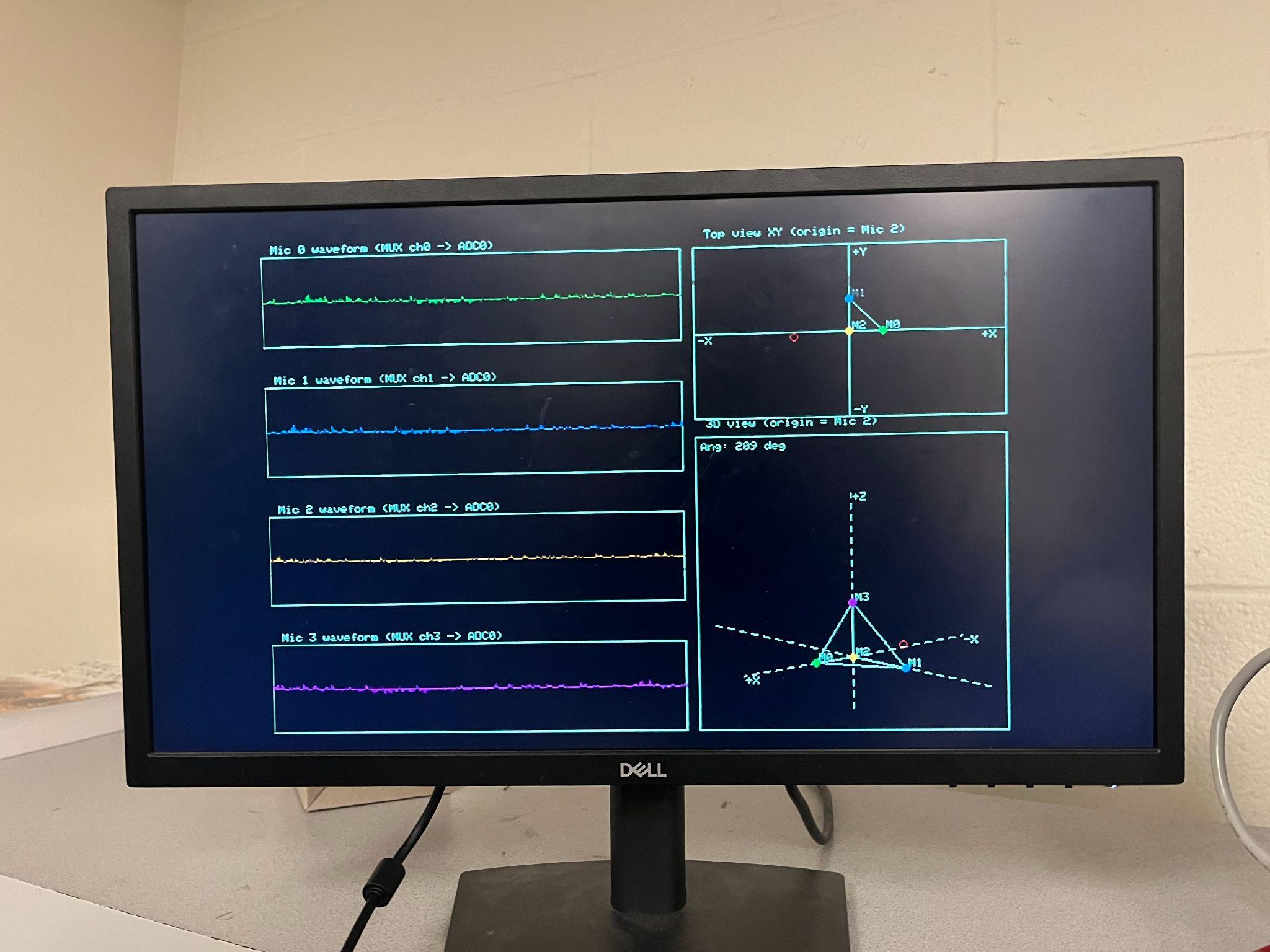
The system was designed to align closely with the core themes of the course, including real-time embedded computation, multi-core concurrency, signal processing, and graphical visualization. Four microphone channels are sampled at 10 kHz, and acoustic events are detected and processed to compute six pairwise TDOA measurements. These measurements are used to estimate a three-dimensional sound source position, which is then displayed in real time as both a 2D top-down view and a rotating 3D visualization. At the same time, raw microphone waveforms are shown on the display, enabling direct correlation between the input signals and the resulting localization output.
This project was conceptually inspired by prior course projects that explored microphone-array-based sound localization and real-time visualization on embedded platforms, particularly the Spring 2025 ECE 4760/5730 project "Audio Localization with Raspberry Pi Pico" developed by Sam Belliveau et al. That project demonstrated event-based audio detection and spatial estimation using multiple microphones. Building on these ideas, our work extends the approach toward full three-dimensional localization and improved spatial interpretability. Specifically, we employ a four-microphone array to estimate six pairwise time-differences-of-arrival (TDOAs) and recover a 3D sound source position using a grid-search-based formulation. In addition, the system provides continuously updated VGA visualization that integrates raw microphone waveforms with both 2D and rotatable 3D spatial views, allowing users to directly observe how acoustic timing differences map to estimated source locations.
Building on these ideas, our work extends the approach toward full three-dimensional localization and improved spatial interpretability. Specifically, we employ a four-microphone array to estimate six pairwise time-differences-of-arrival (TDOAs) and recover a 3D sound source position using a grid-search-based formulation. In addition, the system provides continuously updated VGA visualization that integrates raw microphone waveforms with both 2D and rotatable 3D spatial views, allowing users to directly observe how acoustic timing differences map to estimated source locations.
2.2 Background Math
Sound source localization using a microphone array exploits the fact that an acoustic wave reaches spatially separated microphones at different times. These time differences depend on the microphone geometry and the three-dimensional position of the sound source, which is modeled as an unknown point $\mathbf{s} \in \mathbb{R}^3$. The microphone positions $\mathbf{m}_i$ are assumed to be known and fixed.
Under free-field propagation and assuming a constant speed of sound $c$, the signal arrival time at microphone $i$ is modeled as:
$$t_i = t_0 + \frac{\|\mathbf{s} - \mathbf{m}_i\|}{c}$$
Here, $t_0$ is the unknown emission time of the sound event. Because this emission time is not observable, absolute arrival times cannot be directly used for localization.
To eliminate the unknown emission time, time-difference-of-arrival (TDOA) measurements are computed between microphone pairs. For microphones $i$ and $j$, the TDOA is defined as:
$$\Delta t_{ij} = t_i - t_j$$
Substituting the propagation model into the TDOA definition yields:
$$\Delta t_{ij} = \frac{\|\mathbf{s} - \mathbf{m}_i\| - \|\mathbf{s} - \mathbf{m}_j\|}{c}$$
This expression directly relates the unknown source position to measurable time delays. With four microphones, six independent microphone pairs provide sufficient constraints for three-dimensional localization.
In a sampled system, TDOAs are estimated from discrete-time microphone signals using cross-correlation. For signals $x_i[n]$ and $x_j[n]$, the cross-correlation function is defined as:
$$R_{ij}[k] = \sum_n x_i[n] \, x_j[n + k]$$
The estimated delay corresponds to the lag that maximizes the magnitude of the cross-correlation:
$$\hat{k}_{ij} = \arg\max_k |R_{ij}[k]|$$
The corresponding TDOA estimate is obtained by converting the lag to time using the sampling frequency $f_s$:
$$\hat{\Delta t}_{ij} = \frac{\hat{k}_{ij}}{f_s}$$
To estimate the source position, a least-squares grid search is performed over a discrete set of candidate locations $\mathbf{s}_g$. For each candidate, the predicted TDOAs are computed as:
$$\Delta t_{ij}^{(g)} = \frac{\|\mathbf{s}_g - \mathbf{m}_i\| - \|\mathbf{s}_g - \mathbf{m}_j\|}{c}$$
An error function is constructed by summing the squared differences between measured and predicted TDOAs:
$$E(\mathbf{s}_g) = \sum_{i \lt j} \left( \hat{\Delta t}_{ij} - \Delta t_{ij}^{(g)} \right)^2$$
The estimated sound source position is selected as the grid point that minimizes this error function:
$$\hat{\mathbf{s}} = \arg\min_{\mathbf{s}_g} E(\mathbf{s}_g)$$
2.3 Logical Structure
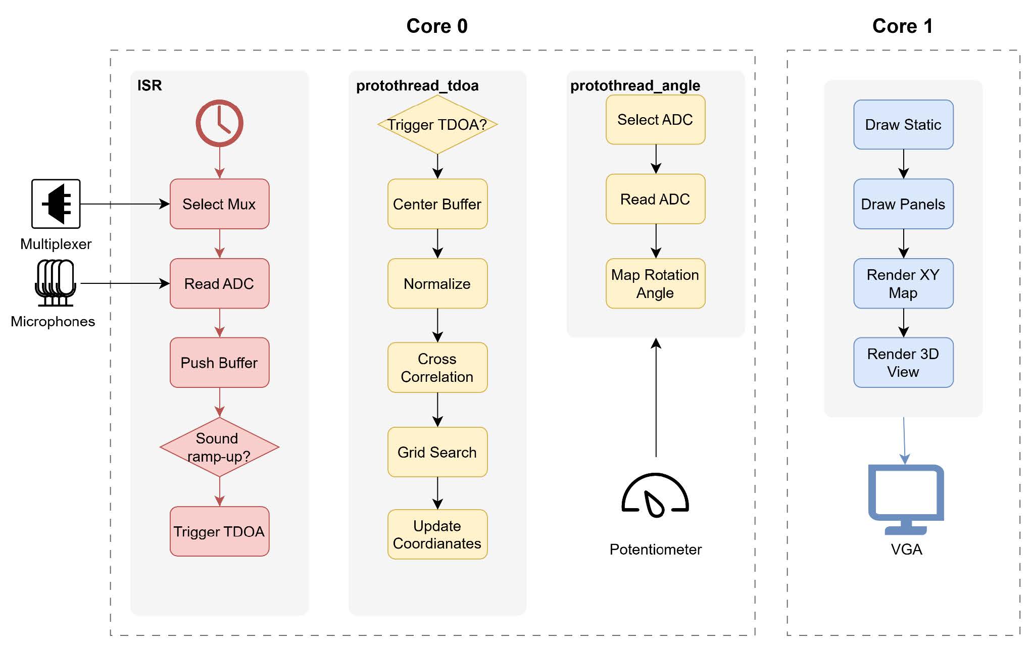
The software is divided into three main subsystems that run across the RP2040’s interrupt handler, two protothreads, and a VGA rendering core.
The timer-based ISR samples four microphones through a CD4051B multiplexer at 10kHz. In each sampling, ISD stores the data in ring buffers, tracks signal energy, and triggers a TDOA event when all microphones detect a sound at nearly the same time. The protothread_tdoa task then copies the buffered samples, removes DC, normalizes the signals, computes cross-correlations, and performs a 3D grid search to estimate the sound source position. The protothread_angle task reads a potentiometer and applies low-pass filtering to determine the viewing angle for visualization. Core 1 handles all VGA drawing, including microphone waveforms, a 2D XY map, and a rotatable 3D view that uses shared state from the main core.
2.4 Hardware / Software Tradeoffs
A key design tradeoff in this project involves the choice of audio sampling rate versus computational load. A sampling rate of 10 kHz was selected as it provides sufficient temporal resolution to resolve inter-microphone delays on the order of a few milliseconds, which is appropriate for the physical spacing of the microphone array. With a maximum correlation lag of ±30 samples, the system can capture up to ±3 ms of arrival-time difference while keeping the interrupt service routine and downstream processing manageable. Higher sampling rates would increase timing precision but would significantly raise interrupt frequency and processing overhead, making real-time operation more difficult on the RP2040.
Another important tradeoff is between continuous localization and event-triggered computation. Rather than performing cross-correlation and localization continuously, the system uses energy-based detection to identify salient acoustic events and only performs TDOA estimation when all four microphones detect an event within a short time window. In addition, a minimum interval of 0.1 seconds is enforced between successive localization events. This strategy greatly reduces unnecessary computation, prevents repeated triggering from echoes or sustained noise, and ensures that expensive operations such as cross-correlation and grid search do not overwhelm the processor.
The choice of a grid-search-based localization algorithm represents a tradeoff between computational efficiency and robustness. Closed-form geometric solutions or lookup-table-based approaches can be efficient under ideal conditions but tend to be highly sensitive to measurement noise, synchronization errors, and modeling inaccuracies. In contrast, a grid search evaluates a physically meaningful error function over a finite spatial region and selects the position that best matches the observed TDOA measurements. Although this approach is computationally more intensive, it is simple to implement, tolerant of noise, and well-suited to an event-driven execution model on an embedded system.
We adopt a dual-core architecture to keep visualization responsive while preserving timing fidelity in signal processing. Core 0 handles interrupt-driven sampling, event detection, TDOA estimation, and 3D localization. Core 1 is dedicated to VGA rendering at a steady frame rate, reading only a small set of shared state variables (estimated position, waveforms, and view angle). This separation prevents the graphics loop from delaying time-critical sampling and avoids visible jitter during correlation and grid-search computation.
2.5 Copyrights
This project makes use of several external software components that are commonly employed in embedded systems coursework. The VGA display functionality is implemented using the vga16_graphics_v2 library, which provides basic drawing primitives and display support for the RP2040 platform. This library is distributed as part of the course infrastructure and is used with proper attribution. In addition, the project relies on the Raspberry Pi Pico SDK for low-level hardware access and on the provided protothreads framework (pt_cornell_rp2040_v1_4.h) for cooperative multitasking and multi-core execution. All application-specific logic, including energy-based event detection, time-difference-of-arrival (TDOA) estimation, three-dimensional grid-search localization, user interface layout, and event-triggered processing, was designed and implemented by the project team.
The signal processing techniques used in this project, such as microphone-array-based localization, cross-correlation for delay estimation, and TDOA analysis, are well-established methods in the signal processing and acoustics literature. In particular, no specialized or patented localization methods are used. The work is intended solely as a non-commercial educational prototype developed within the context of a university course.
Several components and platform names referenced in this report, including CD4051B, RP2040, Raspberry Pi, and MAX4466, are trademarks or product names associated with their respective manufacturers. These names are used strictly for descriptive and educational purposes to identify the hardware components employed in the system. Their inclusion does not imply any endorsement, sponsorship, or affiliation by the trademark holders.
3. Program / Hardware Design
3.1 Hardware and Physical Set-up
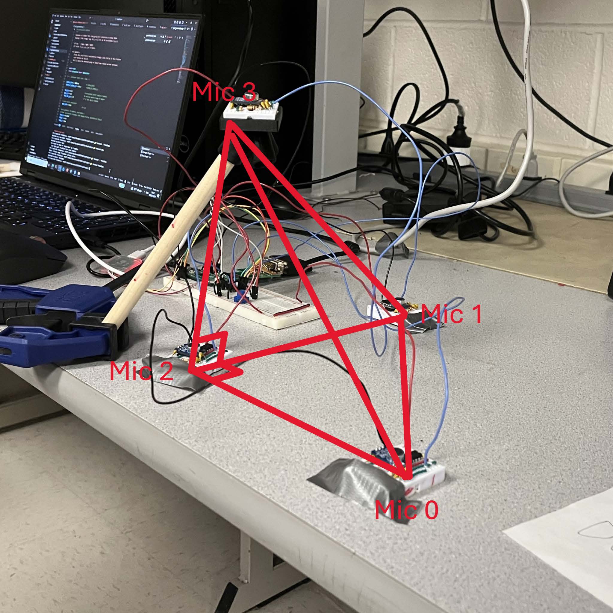
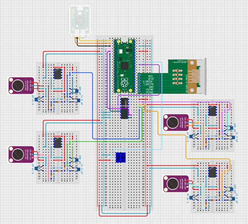
To enable the physical setup required for 3D localization, four microphones were arranged in a tetrahedral configuration. One microphone was designated as the origin, with the remaining three positioned 20 cm away at distinct vertices of the tetrahedron. Each microphone was mounted on a mini breadboard and equipped with a hardware low-pass filter. The four microphone modules were then connected to a central breadboard housing the Raspberry Pi Pico, debugging interface, multiplexer, and a potentiometer for user input.
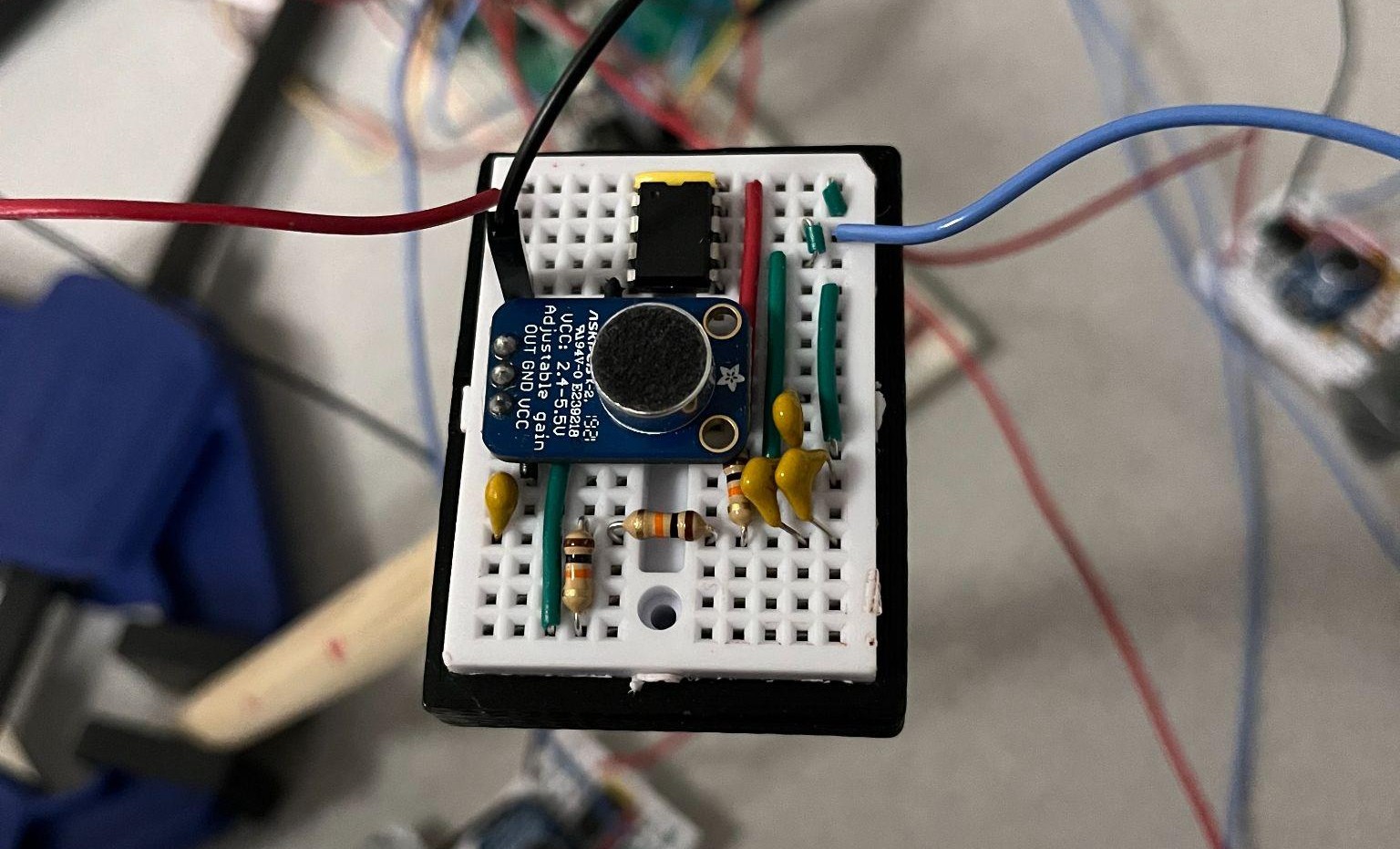
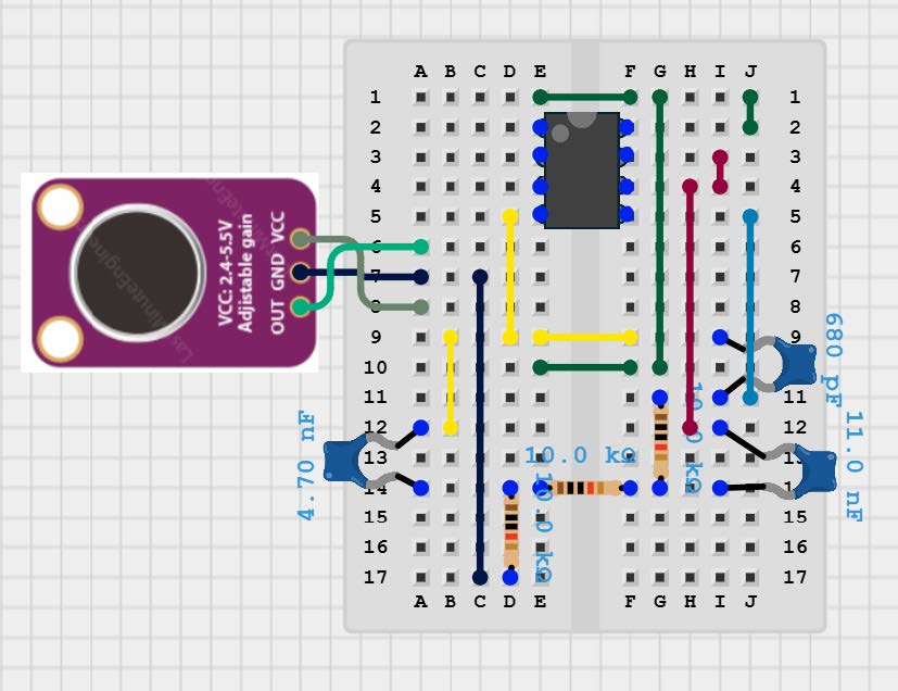
The MAX4466 gain-adjustable microphone served as the primary component of each mini breadboard. Following guidance provided by Adafruit, the microphones were powered using a 3.3 V supply to provide the quietest voltage source. Power, ground, and output connections were made accordingly. The gain was kept consistent across all microphones to ensure uniform signal scaling and reduce variability between channels, which is important for maintaining reliable timing and amplitude comparisons during sound localization. The output of each MAX4466 microphone was routed directly into the input of a three-pole low-pass filter.
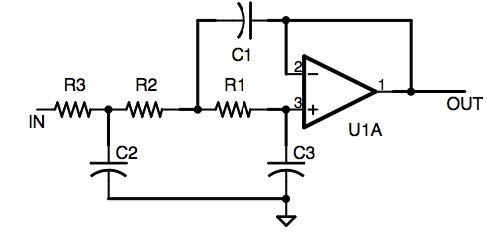
A three-pole low-pass filter with a cutoff frequency of 5 kHz was used to attenuate high-frequency noise while preserving normal sounds relevant for processing. The Raspberry Pi Pico ADC was configured with a 10 kHz sampling frequency, resulting in a Nyquist frequency of 5 kHz. The filter cutoff was set at this frequency to prevent aliasing and preserve signal integrity during sampling. The filter was configured based on the circuit shown in Figure X and implemented using three cascaded RC stages. Equal resistor values were used for all stages (R1, R2, and R3 = 10 kΩ), while the capacitor values were selected to shape the overall frequency response (C1 = 4.7 nF, C2 = 11 nF, and C3 = 680 pF). The three-pole design provided a steeper roll-off than a single-pole filter, improving attenuation of unwanted high-frequency components. Filter performance was verified using an oscilloscope and waveform generator to ensure consistency and accurate low-pass behavior across all channels.
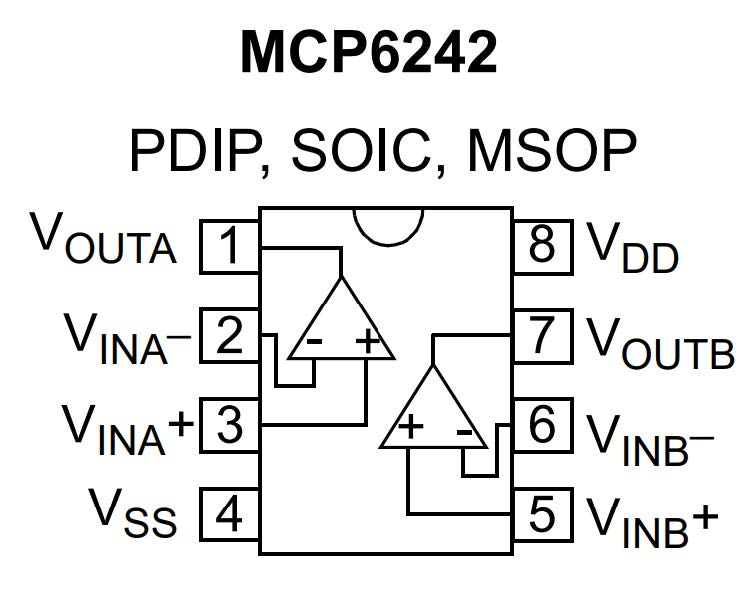
The active filter stage was implemented using an MCP6242 operational amplifier. Although the MCP6242 contains two output channels, only $V_{OUTB}$ was utilized. While the op-amp can operate at supply voltages as low as 1.8 V, it was powered at 3.3 V to match the system voltage and simplify integration with the remaining circuitry.
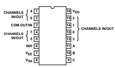
Because the Raspberry Pi Pico provides only three built-in ADC channels, an external multiplexer was used to route all four microphone signals into a single ADC input (ADC0) for consistency. Each mini breadboard was connected to the main breadboard through an 8:1 CD4051B multiplexer, with channels 0 through 3 assigned to the four microphones. GPIO pins 2 through 4 were used as select lines to control which microphone signal was routed to the ADC at any given time. Using a single ADC channel ensured consistent sampling conditions across all inputs and minimized channel-to-channel variation introduced by the microcontroller.
3.2 Multiplexer-Based Four-Microphone Sampling
The program uses a CD4051B multiplexer to read four microphones through a single ADC channel. During each sampling cycle, the ISR selects one microphone by calling mux_select(ch), which updates the three GPIO address lines of the multiplexer.
A critical step in this process is the throwaway adc_read() performed immediately after each channel switch. In the early tests, the microphones appeared to interfere with one another. When one microphone was tapped, another microphone that was far away sometimes produced a similar spike. This effect occurred because the ADC sample and hold capacitor and the multiplexer’s internal switches retained residual charge from the previously selected channel. After the channel changed, the ADC input needed a brief moment to settle to the true voltage of the new microphone. The first reading often reflected leftover charge rather than the new signal. By discarding this unstable reading and using the second one, the program ensures that each stored sample represents the correct microphone and that cross-channel contamination is removed.
3.3 Sound Detection
The system detects a sound ramp by comparing the short-term energy of each microphone with an estimate of the normal background level. Each incoming sample is squared and blended into a fast energy estimate, and the baseline is updated much more slowly to represent typical ambient noise. When the fast estimate rises far above the baseline and also exceeds a minimum threshold, the software marks that microphone as having detected a sound event . This method allows the system to identify quick increases in amplitude that correspond to real acoustic impulses and to ignore low-level noise.
3.4 TDOA Calculation
The system keeps all microphone samples in a circular ring buffer that constantly replaces the oldest entries with new data. The sampling interrupt updates the write index each time it stores one sample per channel, which ensures that the buffer always holds the most recent audio window for all four microphones . When a sound event appears on every channel, the software copies a fixed block of samples from the ring buffer to create four synchronized waveforms. The TDOA routine then removes DC, normalizes the signals, and computes cross correlations for each microphone pair. Cross correlation is evaluated over a range of integer lags using
$$C_{xy}(\ell) = \sum_{n} x[n],y[n+\ell]$$
where $\ell$ is the candidate time shift between two channels. The lag that produces the largest absolute correlation value is taken as the TDOA for that pair. After all six TDOAs are found, the system compares them with theoretical delays across a 3D search grid and selects the point whose predicted delays minimize the total squared error. This point becomes the estimated source location. At the beginning of development, we also tested the GCC-PHAT method, which applies phase weighting in the frequency domain. Details will be discussed in the "Things We Tried But Didn't Work" section.
3.5 Grid Search for Sound Source Estimation
The system determines the sound source location by comparing the measured TDOAs with the theoretical delays that would occur at different points in space. A 3D grid is defined over the region of interest, and each grid point represents a candidate source position. For every point, the software computes its distance to each microphone and converts those distances into theoretical arrival times:
$$t_i=\frac{d_i}{c}$$
where $d_i$ is the distance to microphone $i$ and $c$ is the speed of sound. The expected TDOA between microphones $i$ and $j$ is
$$\Delta t_{ij}=t_j - t_i .$$
These theoretical delays are converted into sample lags and compared with the measured TDOAs. The error for a grid point is computed by summing the squared differences:
$$E = \sum_{(i,j)} \left( \Delta t_{ij}^{\text{meas}} - \Delta t_{ij}^{\text{theory}} \right)^2 .$$
The software evaluates this error for every grid point and chooses the point with the smallest value as the estimated source location. At the beginning, we also tried to replace this grid search with a predefined lookup table to reduce the searching time. Details will be discussed in the "Things We Tried But Didn't Work" section.
3.6 Visualization
The program renders the microphone geometry and the estimated sound source inside a real-time rotatable 3D view. All 3D coordinates come from shared variables, and Core 1 applies a transformation before drawing them on the VGA display. The first step is a rotation around the Z-axis using the viewing angle $\theta$, which is derived from the potentiometer. The rotation transforms any point $(x, y, z)$ into new coordinates
$$x' = x\cos\theta - y\sin\theta$$
$$y' = x\sin\theta + y\cos\theta$$
$$z' = z$$
The program then applies an isometric projection to convert the rotated coordinates $(x', y', z')$ into screen coordinates $(s_x, s_y)$. The projection uses
$$s_x = c_x + k_1 x' - k_2 y'$$
$$s_y = c_y - k_3 z' - k_4 y'$$
where $c_x$ and $c_y$ define the projection center, and $k_1$, $k_2$, $k_3$, $k_4$ control scaling along each axis. This projection provides a sense of depth without requiring expensive perspective calculations. After computing $(s_x, s_y)$ for microphones and the estimated source, the program draws points and auxiliary lines to produce an intuitive 3D visualization that updates smoothly as $\theta$ changes.
4. Things We Tried But Didn’t Work
4.1 Physical Structure and Sound Reflection
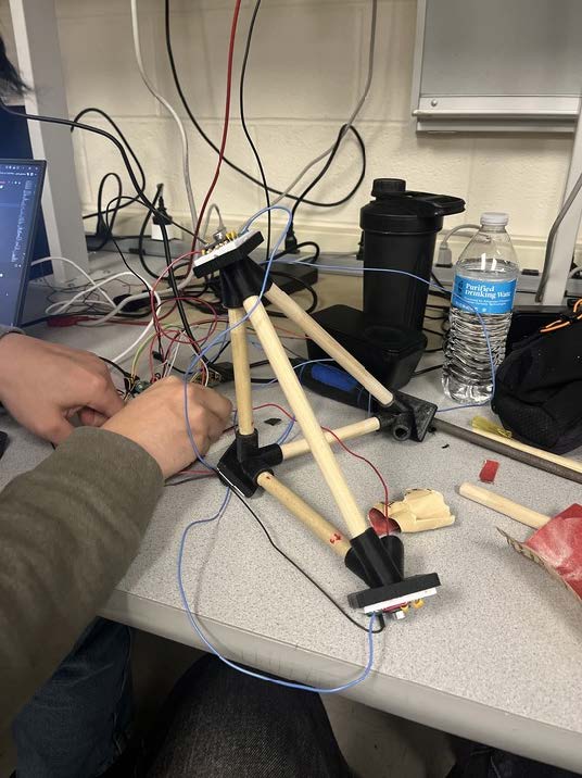
At the beginning of the project, we planned to 3D-print a rigid structure that would hold the four microphones at fixed positions. We experimented with two different frameworks. The first attempt used a regular tetrahedron. We tested its 2D performance by placing the three base microphones in an equilateral-triangle layout and evaluating the 2D localization results. The output was highly unstable. A major reason was the large number of symmetric TDOA patterns produced by this geometry. Several microphone pairs had equal or mirror-image path differences, which caused different source locations to generate nearly identical sets of TDOAs. This symmetry made the system unable to distinguish between many candidate points, and small measurement errors often pushed the solver toward incorrect positions. Due to this fundamental geometric ambiguity, we abandoned the regular tetrahedron design and switched to a triangular tetrahedral framework.
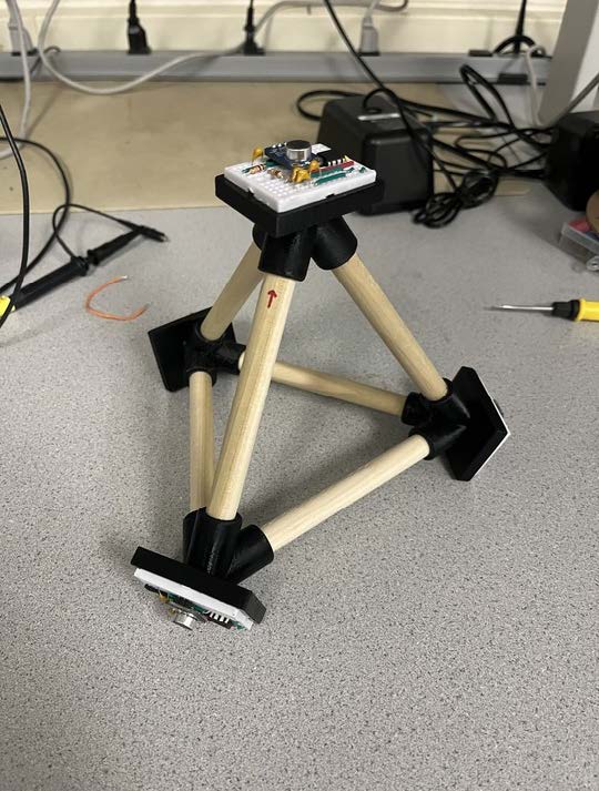
When testing the trirectangular tetrahedron, we again observed very poor accuracy. After two full days of careful debugging, we determined that the problem did not come from the framework's geometry but rather from the physical structure itself. The microphones were connected by 3D-printed parts and wooden rods, and these elements created reflections, resonances, and mechanical coupling that introduced significant acoustic interference. To verify this hypothesis, we removed all structural components. We taped the three base microphones directly onto the table, facing upward, and supported the top microphone on a single slanted wooden stick without enclosing it. This simplified arrangement dramatically improved the accuracy. The reduction in unwanted reflections and mechanical coupling allowed the microphones to behave independently and produced clean TDOA measurements suitable for reliable 3D localization.
4.2 GCC-PHAT Attempt and Practical Limitations
At the beginning of the project, I experimented with the GCC-PHAT algorithm as an alternative way to estimate TDOA. GCC-PHAT computes the cross-correlation in the frequency domain and emphasizes phase information to make the correlation peak sharper in noisy environments. The method starts by taking the FFT of both microphone signals, then forms the generalized cross-spectrum
$$G_{xy}(k) = X(k),Y^{*}(k)$$
and applies PHAT weighting
$$W(k) = \frac{G_{xy}(k)}{\lvert G_{xy}(k)\rvert}$$
to retain only the normalized phase. The TDOA is then taken from the inverse FFT:
$$R_{xy}(\ell)=\text{IFFT}\{W(k)\}.$$
In theory, this approach improves robustness when signals are noisy or reverberant. In practice, it did not noticeably improve detection for this system. The RP2040 must compute multiple FFTs for several microphone pairs, and this cost made localization much slower. Because the time resolution and noise characteristics were already adequate, the simpler time-domain cross correlation provided better performance for real-time operation.
4.3 Early Lookup-Table Approach
At the beginning of development, I attempted to replace the full 3D grid search with a predefined lookup table. A Python script enumerated every grid point and computed its six theoretical TDOAs. For each point, the script created an entry of the form
$$\bigl(\Delta t_{01}, \Delta t_{02}, \Delta t_{03}, \Delta t_{12}, \Delta t_{13}, \Delta t_{23}\bigr) \longrightarrow (x,y,z)$$
where the six TDOAs were integer-rounded and used as the dictionary key, and $(x, y, z)$ was the coordinate associated with that key. In theory, this lookup table produces the same output as grid search and reduces runtime from $O(N^3)$ to $O(1)$.
In practice, the table almost never returned a valid match. Even small measurement errors in any one of the six TDOAs produced a key that did not exist in the table. Integer rounding during table construction introduced additional mismatch and made exact lookup even less reliable. Since the brute-force grid search runs fast on the RP2040 and does not introduce noticeable delay, the lookup-table method was eventually abandoned.
5. Results
The final project resulted in a fairly accurate 3D localization system, which was thoroughly tested by clapping at different locations around the tetrahedral microphone structure. During development, testing was performed at various stages to ensure consistency across microphones, evaluate the system in a 2D orientation, and identify weak points in the design, such as sound reflections caused by earlier versions of the tetrahedral supports. Some of these early tests also influenced features in the final user interface. For example, microphone waveforms were initially used for diagnostic purposes but were ultimately incorporated as a design feature in the VGA display.
Although it is difficult to quantify the exact accuracy of a system like this, it reliably provides a moderately precise sense of the direction of noise-triggered events. The system is highly accessible, offering a low barrier to use and an engaging, interactive way to observe real-time sound localization. The potentiometer adds an additional layer of interactivity, allowing users to rotate the 3D display on the VGA interface, further enhancing the experience and usability of the system.
6. Conclusion
Ultimately, our design successfully achieved the goals outlined in the original project proposal. The tetrahedral arrangement of the four microphones enabled the system to capture precise time-of-arrival differences from multiple directions. This configuration allowed us to develop a three-dimensional localization system capable of determining sound positions in real time. After exploring several approaches, we found that analyzing filtered incoming audio data and applying time-difference-of-arrival (TDOA) calculations produced reliable localization results, which were visualized through a VGA interface.
The VGA interface provided a user-friendly experience, displaying both 2D and 3D projections of the localized sound sources. A potentiometer allowed users to rotate the 3D projections for improved spatial visualization. With additional time, we hope to adapt this system for conservation and citizen science applications. Future expansions could include triggering localization based on specific animal calls rather than a simple noise threshold. Such a system could track animal migrations in real time in marine environments or serve as a tool to assist both novice and experienced birders in terrestrial settings.
7. AI Usage Discussion
AI tools were used as a supplementary resource for concept clarification and writing refinement. During development, we used AI assistance to review and summarize background ideas (e.g., TDOA, cross-correlation, and grid-search localization) and to improve the clarity and organization of this report. AI was also used to brainstorm alternative approaches (such as GCC-PHAT or lookup-table indexing), which we independently implemented in prototypes and evaluated on the RP2040; these alternatives were ultimately rejected due to runtime cost or poor robustness in our measured data. All final implementation decisions, code, experiments, and reported results were produced and validated by the project team. No AI-generated code was incorporated verbatim into the final system without manual understanding, modification, and testing by the authors.
In some cases, AI assistance was used to suggest possible optimizations or alternative approaches, such as frequency-domain correlation or lookup-table-based localization. These ideas were experimentally evaluated by the project team and ultimately rejected when they did not meet real-time performance or robustness requirements on the RP2040 platform. All final algorithmic decisions and implementations were made by the team based on experimental results and direct testing.
In addition, AI tools were used to improve the clarity and organization of the written report. Draft sections were reviewed and refined for technical accuracy, clarity of explanation, and consistency with course reporting standards. All technical content, experimental observations, design tradeoffs, and conclusions were verified and validated by the project team. No AI-generated code was directly incorporated into the final system without thorough understanding, testing, and modification by the authors. The use of AI tools was limited to supportive roles and did not replace original design, implementation, or experimental evaluation performed by the team.
8. Appendix A (permissions)
The group approves this report for inclusion on the course website.
The group approves the video for inclusion on the course YouTube channel.
9. Additional Appendices
GitHub RepositoryDemonstration Video on YouTube
Other references: