Off-grid Diffusion Limited Aggregation on Memory and a Computation Constrained Microcontroller
Project Introduction
As part of our ECE 4760 final project, we created a cyclic Diffusion Limited Aggregation (DLA) simulator that can be controlled via hand motions.
DLA is the process that simulates particles undergoing Brownian motion that form clusters and aggregate upon collisions. Our inspiration for this project comes from both the beautiful shapes that DLA creates and the interesting natural processes that DLA models. DLA also has a multitude of scientific applications, such as modeling snowflakes, crystals, or chemical reactions. Further, we wanted users to be able to interact with characteristics of the DLA algorithm to observe how slight modificactions to parameters can have large downstream effects to emergent behavior.
We implemented two versions of DLA on a RP2040 microcontroller: basic off-lattice DLA, where particles stick infinitely upon aggregation, and cyclic DLA, where particles decay upon aggregation. The simulation is then displayed, real-time, on a screen via a VGA interface. The user is able to interact with the simulation using hand motions by wearing a glove with an IMU attached. Shaking and tilting their hands in various directions will cause the particles to aggregate faster or move with a bias in certain directions.
The following details the design of our simulator, the testing and performance of our system, and some takeaways from the project.
High Level Design
Rationale and Background
Brownian Motion
DLA models aggregate particles whose primary motion is Brownian. Particles undergoing brownian motion can be modeled by moving an amount that is described by a normal distribution whose variance is proportional to time elapsed.
In particular, linear Brownian motion is defined (see page 21) as motion such that for a timestep $h$ the movement of a particle described by $B(t+h) - B(t)$ is normally distributed with mean 0 and standard deviation $h.$ More explicitly this increment $X$ must be obtained with probability $$P(X=x)=\frac{1}{h \sqrt{2\pi}}e^{-\frac{1}{2}(\frac{x-0}{h})^2}.$$ We note that for our purposes $h$ is arbitrary, and dependent on our method of simulation and random number generation.
IMUs
Inertial measurement units measure the acceleration and rotational velocity they experience. With the help of some trigonometry and filtering, it is possible to determine the orientation of an IMU.
With this in mind, we set off to build a motion-controlled DLA simulator.
At a high level, our design involves 3 components:
- The RP2040 microcontroller
- The IMU
- The VGA display
The IMU measures its orientation, the VGA displays the simulation, and our RP2040 both simulates and interfaces with the IMU and VGA. The mean and variance of the normal distribution used to model particles' behavior could be changed depending on the orientation and acceleration of the IMU. Concretely, this meant that we could bias particles to, on average, move in a certain direction, as well as control the simulated speed at which the particles were moving.
Hardware/Software Tradeoffs
One place we encountered some tradeoffs involves the polling rate of the IMU. To an extent, we could increase the responsiveness and accuracy of our orientation measurements by polling the IMU more rapidly. However, polling the IMU takes a nontrivial amount of time. In particular, time spent reading from the IMU is time not spent simulation particle motion. After a certain point, a high polling rate led to both undesired behavior and even crashes. This is expanded upon below. We decreased the polling rate of the IMU to avoid these issues.
Another tradeoff we dealt with involved the amount of bits used to describe a pixel's color. We were concerned that using 8 bit color (i.e storing the color as a char) would make us run into memory size limitations. For this reason we used 4 bit color in our program. While it turns out that we probably would have been fine using 8-bit color, as the number of particles we used was limited by their density in our "screen-space," we had at this point made some implementation choices that would have made it difficult to transition to using 8-bit color. For this reason, we continued using 4-bit color for our project.
Existing Patents, Copyrights, and Trademarks
Regarding patents, copyrights, or trademarks, as far as we know none are applicable to this project. We've sourced all online coding resources that inspired us/were used for reference. Much of this work was enabled by some of Bruce Land's C PICO SDK work, without his protothread and VGA drivers this project would have been out of scope for the 5 weeks we had to complete it.
Design
Hardware
The heart of our system is a Raspberry Pi Pico, which features the RP2040 microcontroller. We implemented the circuitry for this lab using a breadboard, shown below Fig 1. Similar to previous labs, our microcontroller communicates through UART to interface with a PuTTY terminal serial interface and utilizes the Pico's PIO state machines (see chapter 3) to implement VGA drivers that allow us to visualize our simulation.
Figure 3 below visualizes how we integrated the VGA display, RP2040, IMU (MPU 6050), and Serial interface (USB-A and PuTTY terminal) together.
To allow for 4 bit color with a green gradient, the VGA connection utilizes a summing circuit, as seen in Figure 3 above. We use four resistors with the approximate resistances 1R, 2R, 4R, and 8R where R $\approx$ 100, based on the resistors we had available in the course lab. Looking at Figure 3, we see that if we set all four GPIOs to high, we get the brightest green, whereas if we only set the rightmost GPIO to high, we get the dimmest green.
Software
The software we built for our simulator can be broken into a number of components. We will describe each component as it stands alone, and then describe how these components integrate together.
Random number generator
Simulating brownian motion requires drawing from a normal distribution. Most modern languages have implementations of functions that do this built in to their standard libraries.
C, however, lacks such functionality.
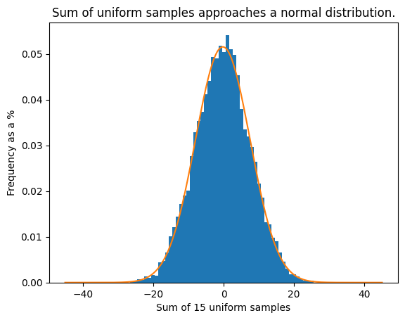
What C does offer is a rand() function that returns a value sampled from a uniform distribution between 0 and some constant RAND_MAX. We use this uniform distribution to approximate a normal distribution by drawing from rand() multiple times and updating a particle based on that value. Over many time steps, the motion of a given particle will approximate a normal distribution as a result of the Central Limit Theorem. As our particles are updated 30 times a second, and the sampling distribution tends to normal over time, we can get a good approximation of brownian motion with this uniform distribution. Figure 4 shows the empirical probability distribution of displacement of a particle over 15 timesteps (equivalent to half a second), using this "sum of uniform samples" method. Figure 5 shows the empirical probability distribution of displacement of a particle over 15 timesteps sampling from a normal distribution at each time step. The distributions between each method are very similar, with our uniform distribution method being slightly biased towards the right. We believe this is an artifact of the visualization of our as our uniform distribution has integer values, and our simulation did not show any obvious tendency to positive values at runtime. The takeaway from this graph is that, over time, our particles behave as if they were moving randomly with movement at each timestep being samples from a normal distribution.
Particle State and Collision Detection
Our particles consisted of x and y coordinates stored as shorts, color stored as a char, and a cyclic_counter that tracked how long a particle was aggregated for. In order to minimize memory usage, our color member variable also acted as a way to determine if a particle was aggregated or not. Particles that were not aggregated had a color of either 1 (dimmest possible green) or 0 (black), while particles that were aggregated had colors ranging from 2-15, (increasingly bright shades of green). All particles were stored in an array.
Collision detection was implemented by with the help of fixed point precision types, with 16 decimal places, a alpha max beta min square root approximation algorithm, and our pixel backing array.
Our collision detector calculates the distance between a particle's current location and its new desired location using the alpha max beta min algorithm. It then uses this distance to determine an increment, which can be thought of as a vector of unit length in the direction of the particles updated location. With the help of this "increment vector", each pixel in between the particle's current location and new location is checked to see if it is touching existing aggregate or not. If a pixel is determined to be touching our aggregate, the particle is moved to that pixel (falling short of the intended update location) and it is mutated to be part of the collective aggregate (by changing its color to bright green). If the path between a particle's current location and new location is free of aggregate, the particle is moved to the intended update location and remains "active" (as opposed to aggregated).
Touching Aggregate Detection
Recall that our aggregate consists of various shades of green (represented as color values from 2-15). A pixel is deemed to be touching aggregate if the sum of the colors of the 8 pixels surrounding it surpasses some threshold. This threshold can be tuned to change the emergent behavior of aggregation, but was often left at 15 as this often produced interesting results. As an example, with a threshold of 15 a pixel would be deemed to be touching aggregate if it neighbored at least a single "bright green" pixel, or at least 2 pixels with color values of 8 (theoretically, half as bright as a "bright green"), and so on.
Angle detection
The following is adapted from our lab 3 report. And is included here for completeness:
Our raw MPU6050 IMU measurements were received via I2C, where specific registers were read, corresponding with specific measurements of the IMU. While we initially planned to utilize the IMU's raw gyroscope measurements around the x-axis and y-axis to compute rotational deltas, we found that just using accelerometer data proved accurate enough for responsive use. Getting rid of the gyroscopic factor would reduce the computational complexity of our simulation without affecting its quality, so we opted to just use the accelerometer to determine our angle
Our raw accelerometer data was used to compute the angle of our lever based on an inverse tan function (see Figure 6). The raw data from our accelerometer was low passed, as noise in the raw data is amplified through the inverse tan function. See the next section for more information.
Figure 6 shows how accelerometer data can be used to calculate an angle of an IMU. In our case, we were interested in measuring rotation around the x and y axes. Taking the inverse tangent of acceleration in the z direction and the direction that we are not calculating (i.e to determine x-axis rotation we need y-axis acceleration) gives us the rotation around that axis.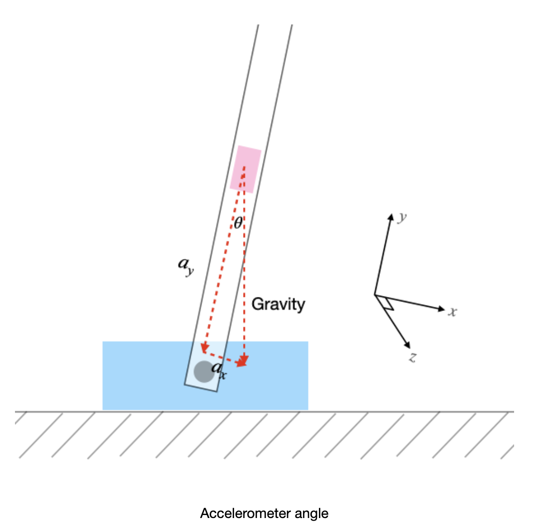
Low pass
The following is adapted from our lab 3 report and is included for completeness:
A software low-pass filter was used on our raw accelerometer data.
This software filter essentially averages our readings in relation to our current data over multiple periods of time, smoothing out any high frequencies. We applied low pass filters to our accelerometer data because the effects of noise would be greatly amplified through an inverse tan function, leading to very noisy angle values.
Acceleration Variance Detection
The variance of the acceleration in the z axis our IMU underwent over a period of 0.66 seconds was tracked. This was accomplished by maintaining a rolling average and storing the previous 20 z-acceleration values obtained from our IMU and calculating the variance of our Z acceleration: $$\text{Var}(Z) = \mathbb{E}[(Z - \mathbb{E}[Z])^2]$$
The variance calculation was performed naively (iterating over all values in our array), but proved fast enough to be computed in the span of a single frame.
Particle Movement
Our particle movement was implemented by moving a particle in the x and y directions an amount obtained by sampling from a uniform distribution. The max_speed variable is dependent on the variance of our z-acceleration. It describes the magnitude of the most a particle could move in a direction. So if max_speed was 6, a particle could never move more than 6 or -6 in either direction.
The mean of this distribution depended on the angle of our IMU. Rotation along the y-axis of the IMU (pointing towards the screen) corresponded with the horizontal movement of our particles, and likewise for the x-axis and vertical movement. The mean of our distributions moved stepwise linearly based on the ratio of the angle of our IMU with 90. Meaning rotation around an axis of 90 degrees had a (absolute) mean of (max_speed - 1) / 2, while a rotation of 0 degrees (i.e the IMU was flat) had a mean of 0.
You may be asking why we set (max_speed - 1) / 2 and not max_speed / 2 when our IMU was fully rotated? This is because if we had set the mean to be exactly max_speed / 2 our particles would have only ever moved in a single direction. This makes the movement seem un-random nature and is not satisfying to interact with. For this reason we enforced the ranges of our uniform distribution to never be higher than -1 and never be lower than 1 (depending on the direction of tilt). This slightly changes the mean of our distribution.
Particle decay
We were interested in simulating cyclic DLA. To this end, our particle structs store a cyclic_counter member variable that counted the number of frames a particle had been aggregated for. The more time a particle had been aggregated for, the dimmer the aggregated particle would appear, before disappearing and returning to be a "free" particle, undergoing Brownian motion independent of the aggregate. This feature is displayed when explaining cyclic factor results.
Simulation/Animation
30 times a second our simulation/animation protothread was awoken. This thread was responsible for polling our IMU, performing collision detection, updating particle locations and colors, and finally writing to our pixel backing-array. While responsible for many tasks, in practice this protothread largely consists of a bunch of function calls in a while loop. Some of these functions are guarded by flags that let us turn features (such as variable speed, tilt bias) on and off.
Serial
Part of our simulation interfaces via UART to a PuTTY terminal to allow us to turn feature flags on and off, and reset our simulation. Serial runs on it's own protothread and utilizes non-blocking serial read and write functions, obtained from Bruce Land's protothreads modifications. These non-blocking functions rely on the RP 2040s ability to signal when UART can be written to. The thread responsible for reading/writing yields until a character can be read/written via UART, and in this way only runs when needed. This allows for computational threads (such as simulator/animator) to run almost constantly.
Bringing it all together
After initializing all of our UART and IMU GPIOs, along with our PIO state machines, our serial and simulation/animation threads are initialized. Our serial thread is non-blocking, and simply uses protothreads to output to terminal and read in to an input buffer as needed. Some logic regarding flags is contained in this thread as well. This thread is initialized on our second core.
Our simulation thread is initialized on our first core. In a given frame this thread polls our IMU and updates the parameters that describe our uniform distribution based on our IMUs acceleration variance and tilt. Then, two samples are drawn from our distribution and fed to our collision detector. Our collision detector updates the location and color of our particle, based on the aggregate currently present (i.e. a particle moves an amount determined by our random sampling, or collides with aggregate in the way). The particle's old location is drawn over ("erasing" it) and the particle's new location is drawn to.
The thread then yields such that it will awaken 1/30th of a second after the current frame begins. In this way we enforce a simulation and animation speed of 30 fps.
Testing
Hardware
We had used the VGA display and the IMU, previously as part of lab 3 of the course. At setup, we had to make sure the connector was wired correctly and that the receiving monitor was functional (which was not always the case). If the receiving monitor did not properly display our program, we knew that either the wiring was incorrect or the monitor had to be swapped out. Luckily, being familiar with the IMU made it easy for us to leverage its acceleration and angle capabilities.
When testing for user input, we wired up the UART connection to input keyboard presses using PuTTY. With this wired up, we set flags enabling/disabling specific features and tested specific elements of our hardware. As we succesfulkly interfaced with our PuTTY terminal, we were confident in the UART implementation we were using.
We did have some difficulty implementing the 4 bit green gradient as it required some additional circuits knowledge. Fortunately, the required summing circuit utilized resistors available in lab and the circuitry was not complicated. That being said, we were able to verify this 4 bit green gradient by using the VGA display and determining whether particles were properly decaying from the brightest green to the dimmest green.
Software
Like previous labs, we utilized serial's print capabilities to allow us to examine the values of variables in real time. Beyond that, a large amount of testing was done by looking at our IMU acceleration and complementary angle graphs to determine whether the particle motion was correct. For the features that did not utilize the IMU, their effectiveness could be verified by looking at the program and comparing it to the expected result.
Angle Graphs
We used software (modified from here) to graph the measured angle of our rotation around both the x and y axis. This allowed us to both examine the behavior of our angle measurements with respect to noise and responsiveness, and qualitatively view the effects of changes we made to our measurement algorithm. In particular, graphing proved invaluable to help us notice that changing our polling rates had down stream effects on measured angles, and required modification to our low pass algorithm to account for these changes.
Furthermore, our graph helped us verify that our parameter changes were behaving as expected. In particular, our graph allowed us to tell at what angle the mean of our uniform distribution shifted (which was a stepwise function). We verified that our mean shifted at the intended angles through user testing.
Simulation
Having an obvious visual component to our simulation made testing for its correctness easy. After making changes to our algorithms, we verified visually if our simulation behaved as expected. We compared our simulation both to other, examples of DLA and to previous iterations of our own work. Examining incremental changes to our simulation algorithms helped us uncover a number of issues, described in detail below. Among the issues we discovered was a shift in the mean of the movement of our particles from conversion from fixed point to integer values, incorrect aggregation occurring at the borders of our simulation, and some issues with a naive collision detection algorithm.
Results
We visually tested our simulation with various features and parameter values. Our initial, basic DLA simulation had no motion controls and simply modeled Brownian motion aggregation of particles. Once that was complete, we tested our tilt, speed, cyclic, visibility, seed location, and reset. We found that for the space allocated in our simulation (an invisible bounding box in the snippets below), 8000 particles proved enough particles to be interesting while not creating too high of a particle density such that aggregation would occur extremely rapidly.
Basic DLA
The basic DLA motion consists of a min speed = -2 and a max speed = 2. As shown below, the clustering motion branches out evenly from the center, and matches the patterns generated by many other DLA simulators (see the References section).
Tilt Factor
Activating our tilt feature shifted the mean of the normal distribution modeling the motion of our particles, and is responsible for creating a slight bias in particles' movements. As shown below, the particles are first provided a bias to the right and then a bias to the left. A common characteristic of the tilt factor is the tendency for particles to clump into high density areas, which aggregate very rapidly once a single part of that "group" reaches some aggregate. This feature can be turned on/off via serial.
Speed Factor
The speed factor, modified by the variance in acceleration in the z-direction, is responsible for increasing the min speed and max speed bounds based on the variance of the z-acceleration. In order words, the movement of the particles will increase depending on how fast the IMU-glove is shaken. This feature was responsible for the conception of the collision detection. Before the collision detection, particles with increased speeds would cluster incorrectly, skipping over aggregate particles rather colliding with them. Now, the particles are capable of reaching max speeds of around 7 As shown below, the particles are first moving very quickly as a response to the real-time IMU-glove movement. Then, the IMU-glove movement is stopped and the particles begin slowing down, showing how the particles' movement responds to dynamic hand motions. This feature is activated via serial.
Cyclic Factor
The cyclic factor is responsible for decaying aggregate particles and randomly respawning them, allowing for continuous simulation. Like the other features, it is activated through serial, but an additional integer is provided to alter the decay rate. In the past, once the particles would all aggregate, the program would have to restart. As shown below, the particles decay at a rapid rate, creating a creeping motion of our aggregate throughout the screen.
Visibility Feature
The visibility feature is responsible for hiding all moving particles, only highlighting the aggregate particles. The result is a cleaner clustering motion as the thousands of moving particles are not shown. As shown below, the basic DLA motion is highlighted without any background movement.
Seed Location
The seed location feature is responsible for adding an aggregate particle seed in a custom location. This custom location is determined in serial based on an input x and y coordinate. The custom seed is a permanent aggregate particle, allowing for more unique patterns.
Reset
The reset serial command is responsible for either committing a hard or soft reset. Turns off all activated features, while a soft reset respawns all particles, separating them from any created aggregate. Shown below is a hard reset.
Maximum of Particles
While we were capable of smoothly running 7000-8000 particles, the program is capable of running 16000 particles based on memory limitations. However, as the particle count increases, there were noticeable reductions in frame rate. This reduction is especially noticeable depending on which factors are activated. Because tilt, speed, and cyclic are computationally intensive, these factors are the computational bottleneck. Additionally, as mentioned above, running the maximum number of particles would also significantly increase the particle density, making all particles aggregate very rapidly.
Safety
There are no significant safety concerns. A minor concern could be that waving one's hand rapidly up and down to alter the variance of z-acceleration could lead to someone getting smacked. Users should be aware their surroundings before controlling the simulation.
Usability
Our program requires users to be able to freely move their hands to use the motion controls. However there are serial based workarounds for this. Unfortunately, the visual component of our simulation would not be very accessible for the visually impaired.
Bugs of Note
We detail below some of the bugs we encountered while building our simulator, how we overcame them, and any takeaways we have.
Rotten Randomness
Before settling on the approach of approximating a normal distribution over time by sampling from a uniform distribution, we attempted a few ways to sample from a normal distribution for every particle, once a frame. One approach involved summing over multiple calls to rand() in order to approximate a normal distribution within a single frame. Because this involved 10s of function calls per particle, it severely limited the speed of our due to the increased computation complexity. Another approach involved sampling a random bit using the RP 2040's ring oscillator clock (ROSC). With these random bits it is possible to generate a wide variety of distributions, including a normal one. Furthermore, it is possible to perform many of the tasks required to generate a normal distribution by utilizing the RP 2040's DMA channels, at little to no cost to the CPU.
While the second approach in particular is attractive due to the minimal cpu overhead, testing found that the simple approach that we went with, generating a normal distribution "over time" simulated well and was both nice to interact with via motion controls, and behaved inline with other DLA simulations. For this reason we were happy to keep using rand() and move on to other parts of our system.
Polling Problems
Initially, polling our IMU at a rate of 1,000 Hz via a repeating alarm timer led to our simulation crashing shortly after startup. It was unclear what the root cause of these issues were, as they persisted even when moving our repeating alarm timer to a different core. Which goes against our initial suspicion that our interrupts were interfering with in-flight writes/reads to our backing pixel array, which may have eventually led to the reading of garbage data which softlocked our program.
To resolve this, we moved our IMU polling trigger to occur within our simulation protothread. This meant that no calculations/pixel updates could be interrupted, and guaranteed the sequentiality of our polling -> simulate step.
Moving our IMU polling trigger to our simulation protothread meant that our IMU was only polled 30 times a second, as opposed to 1,000. However, we found that this frequency still provided accurate enough readings for our motion controls to feel responsive.
Bonkers Borders
In addition to crashes, enabling IMU polling changed the behavior of pixel aggregation, leading pixels to aggregate seemingly at random at the borders of our simulation. This was eventually resolved by adding better bounds logic to our touching-aggregate function. However it remains unclear why polling the IMU changed our collision detection logic.
Aggravating Angle Assessment
During testing, we noticed that if we rotated our IMU to close to 90 degrees along the x-axis, the rotational measurements of our y-axis would become inaccurate. The same occurred if we swapped the axes of rotation. We learned that using acceleration along axes is limited in that at extreme angles we lose a degree of information. Consider rotating around an axis pointed in front of you (y axis pointing forward, x-axis to the left, z-axis pointing towards the sky). Our IMU calculates rotation around the y-axis by comparing z and x-axis accelerations. Consider that if we rotate along the x axis so that our y-axis is now pointing up (z axis pointing towards us, x axis pointing to the left), rotation around the y-axis no longer changes the acceleration experienced in both the x-axis and z-axis, rather, both remain close to 0. This makes measurement of rotation around y very difficult and sensitive to noise.
Luckily for our project, users did not often reach rotations of 90 degrees, as doing so was quite uncomfortable with our glove. So this did not prove an issue in practice.
Takeaway: It was discussed how in measuring rotation around 2 axes, we were essentially trying to model the IMU in 3 degrees of freedom. However, we were doing this with only 2 pieces of data in each axes: z acceleration and x/y acceleration. To this end our measurements were underdetermined, and caused the issues described above. We should aim to have fully determined systems, and if that is infeasibly be aware of the limitations of our models
Restrictive Rounding
When shifting the mean of our uniform distribution based on the tilt of our IMU we performed fixed point arithmetic for the sake of computational speed, and then converted values to integers. Our initial system took into account the sign of our tilt, and shifted the mean of our distribution accordingly, based on the between our current angle and 90 degrees.
Because of the way our fixed to integer conversion works, numbers were rounded differently dependent on their sign. Namely, fixed point representations are converted to integers by right shifting >>. This means that integer values are truncated, not rounded. This meant that we were taking the floor of our fixed point number. This has an effect on the magnitude of a number after truncation based on its sign. Consider that 4.3 is truncated to 4 while -4.3 is truncated to -5. This, along with the details of our initial implementation, meant that our mean was incorrectly being biased towards negative numbers. This was apparent in our simulation as particles tending towards the top left, even when our IMU was held flat.
To fix this, we negated some fixed point numbers before truncating them and negating them again. In this way, our truncation was "symmetric" on both positive and negative fixed point numbers.
Takeaway: Implementation matters! Especially when developing in C on things like microcontrollers, we need to be very aware of the implications of various implementations, as they can have compounding downstream effects. We were fortunate enough to figure out what was going on fairly quickly, but this may had not been obvious if we had been less aware of different number representations and how we convert between them.
Conclusion
Improvements and Extensions
If we were to attempt this lab again, it would be interesting to continue tuning our decay and aggregation parameters that give rise to interesting emergent patterns. We were able to generate crystal-like structures as well as subtle rippling motion, but we were unable to recreate some of the patterns seen here (which helped inspire this project).
We could also extend some of the features we have.
For example, we could implement a "drawing" feature that would allow a custom aggregation seeds to be drawn on the screen based on motion controls and a cursor. The current custom seed feature is only capable of adding a single seed at a time. However, this "drawn seed" could perhaps lead to more complex cluster formations.
For future extensions beyond adding more DLA features, we could expand our program to highlight other particle models as well that go beyond Brownian motion. Though the DLA patterns are interesting, there are many patterns that cannot be replicated using DLA. Things like Laplacian Growth models could be used to simulate crystal growth and electrodeposition. Other mathematical models could be used to simulate fungal growth or bacteria colonies. It would be worth comparing how all the models respond to adding the existing speed, tilt, and cyclic features as well.
It could also be interesting to explore possible optimizations in our drivers that could help us expand our simulation. In particular we used a 320x240 size screen instead of a 640x480 screen due to memory constraints. It would be interesting to try and overcome this limitation to allow for higher resolution simulation.
Final Thoughts
While this project integrated concepts we've learned throughout the semester in a new way, and the DLA modeling itself was the result of our own implementation. We're excited in the future to possibly build more of these components, such as the VGA driver, from scratch.
On a personal note, it was especially exciting to see our program in action. Seeing our project begin as an abstract and then turn into life was particularly rewarding, especially because there were many challenges along the way. The program often created patterns that were unexpected, leaving us mesmerized as we fiddled with parameters of our program.
As mentioned in the previous section it would be interesting (although possibly difficult) to use a more complex model of motion that could potentially lead to more life-like formations.
Intellectual Property
There are no intellectual property concerns we are aware of. We are grateful for Bruce and Hunter's available software libraries.
Appendix
Permissions
Project Website
The group approves this report for inclusion on the course website.
Project Video
The group approves the video for inclusion on the course youtube channel.
Tasks
The work was largely evenly split among team members, with slight focuses on certain. The following is a non-exhaustive list of topics focused on.
Nathaniel: Setup and dev environment, collision detection, voltage divider, website, and report.
Angela: Collision detection, voltage divider, aggregation algorithm, website, and report.
William: Random number generation, motion-random-distribution effects, serial, website, and report.
References
Code
Code can be found here.