This webpage is the final report for our final project in ECE 4760 Microcontrollers Fall 2023.
Project Introduction
For our final project, we built Computron, a parallel computer consisting of Raspberry Pi Picos that communicate over a I2C bus. To demonstrate the power of parallel computation among these devices, the Mandelbrot set is computed across Picos. Every Pico computes a portion of the set, while one is also responsible for projecting the set onto a VGA monitor. This projection unit is special, in that it is the only peripheral device on the I2C bus while every other Pico is an I2C controller. We were able to configure the projection unit to dynamically recognize the number of controllers on the network prior to computation, and to distribute work accordingly without a user informing the network directly. In the end, with eight Picos connected together we were able to achieve about a four-times speedup in computation of the Mandelbrot set compared to computation on a single Pico.
High-Level Design
After completing Lab 2, both of us were still captivated by optimizing the Boids program even further than we were able to initially. Besides implementing more direct software optimizations to put more Boids onto the screen, the idea of running the program across multiple Picos came up. We reasoned that the boost to computation power would offset the incurred communication overhead enough to create a nonnegligible speedup. However, parallelizing the Boids program in particular appeared daunting, due to the problem of sharing all the necessary boid information across Picos in a timely fashion. Moreover, the time constraint of the project itself posed to be a concern. Thus, in large part due to advice from Professor Land, we decided to instead parallelize the Mandelbrot set program from the ECE 4760's demonstration code.
Originally, we did not plan on using I2C as our final communication protocol. Instead, we had planned on using CAN as our network protocol. To us, CAN was a sound compromise between the speed of SPI and the ease of use of I2C. However, because our CAN transceivers came in later than expected, we decided to start our work with I2C. Though we wished to be able to implement our project in both I2C and CAN in order to compare the two, we ended up only having time to implement the I2C version of our parallel computer.
Besides its inherent aesthetic appeal, the Mandelbrot set also serves as an excellent benchmark for parallel computation power, in that its algorithm contains no dependencies between results. This means that work can be done simultaneously on many different devices, and none of them ever rely on the results of another device. To put this into computer architecture language, the algorithm presents no possible data hazards.
From the outset, there was an obvious networking overhead tradeoff that would be incurred as Picos were added to the network. While each additional Pico would afford the network two more cores to use for Mandelbrot computation, it also would further crowd the single I2C bus connecting every device on the network. This meant that doubling the number of Picos would not necessarily halve the computation time for the entire Mandelbrot set, and that at some point we would essentially reach a horizontal asymptote as far as performance went. The severity of this overhead would have likely been diminished if we had decided on a different type of network as well. For instance, a tree-like network of Picos using SPI would probably not see diminishing returns as quickly, because not all devices would share a bus and SPI itself has a greater transfer rate than I2C. However, because of time constraints, we decided that a simpler, single bus I2C network would still function well enough.
Beyond its immediate aesthetic appeal, the Mandelbrot set is interesting primarily because it is the result of relatively simple math. The following equation is the core of the Mandelbrot set, and is applied to points on the coordinate plane:
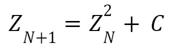
In this equation, Z is a complex number that is equal to zero before its first iteration. C is a constant, complex number that is taken to be the x and y coordinates at that point on the plane (where x is the real component and y is the imaginary component). Though this equation on its own may seem insignificant, what makes it significant is how it is interpreted. Specifically, if Z diverges at a given coordinate, then this point is said to not be contained in the Mandelbrot set. Accordingly, if Z does not diverge and is in fact stable, then the point is contained by the set. Essentially, Mandelbrot at its core is a plot showing which coordinates produce a stable result for the above equation.
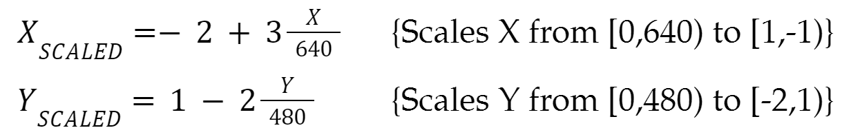
To make this underlying math work efficiently on the Pico, some simplifications and tricks are used. First of all, and perhaps most importantly, testing divergences to infinity is not feasible without limiting the number of iterations done for the Mandelbrot equation to a reasonable number. In the case of our implementation, the Mandelbrot math will only go up to a thousand iterations. Moreover, there must be a threshold magnitude beyond which Z is guaranteed to diverge and thus not belong to the set. In our implementation, this threshold is set to equal two. It is difficult to explain why the number allows for the computation to function correctly, but an intuitive observation to make that may help one understand is that two is the largest number you can subtract from its own square and have a difference less than or equal to that number.
Another mathematical adjustment made to allow the Mandelbrot set to generate properly is the scaling of coordinates. For our implementation, a 640x480 pixel VGA monitor is used for displaying the resulting set. However, for the set to generate cleanly within these bounds the raw pixel coordinates must be scaled. For following equations scale the x and y coordinates so that they properly produce the Mandelbrot set for our purposes:
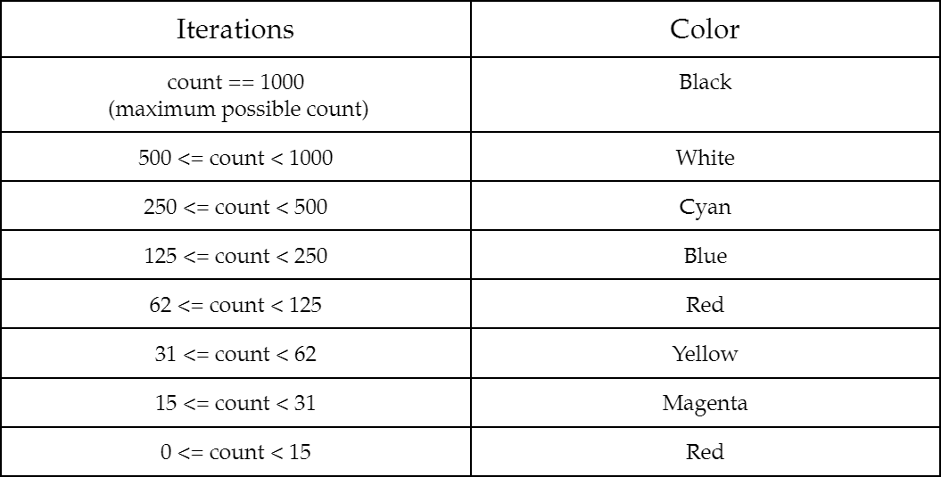
Lastly, the Mandelbrot set is much more interesting when it is not only shown which coordinates diverge and which do not but also how quickly points outside of the set diverge. To demonstrate this, pixels can be colored depending on how many iterations it takes for their coordinates' complex magnitudes to exceed the threshold of two. In the follow table, the way iteration counts determine a pixel's color is explained:
Beyond the math behind the Mandelbrot set itself, our setup logic was also very important, as this determined how work was distributed across Picos. It is because of the way that setup is completed that all Picos except the projection unit are marked as I2C controllers, while the projection unit itself is set as an I2C peripheral. The communication between devices is explained in the following steps:
1. A math unit (I2C controller) takes control of the I2C line shared between all units when it is available, and reads from the projection unit
2. The projection unit writes to this math unit with the total count of Picos on the network thus far. If this is the first math unit to contact the projection unit, for instance, then the count will just be one. This value becomes the ID for that math unit.
3. Once a second has elapsed, it is assumed that the projection unit has the total count of Picos on the network. This unit then writes the total count to all of the math units.
4. The math unit is responsible for computing all columns of the Mandelbrot set whose x coordinates are divisible by the total number of Picos after being already subtracted by the unit's Pico ID. For example, a math unit with an ID of 3 in a network of eight Picos is responsible for columns of x coordinates 3, 11, 19, and so on up until 640. The projection unit is also responsible for computation, and assigns itself with an ID of 0.
5. As pixels are computed on the math unit, if the resulting color is not black then the information for that pixel is written to the central projection unit to be put onto the monitor.
Program/Hardware Design
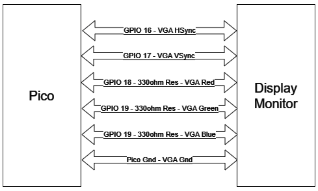
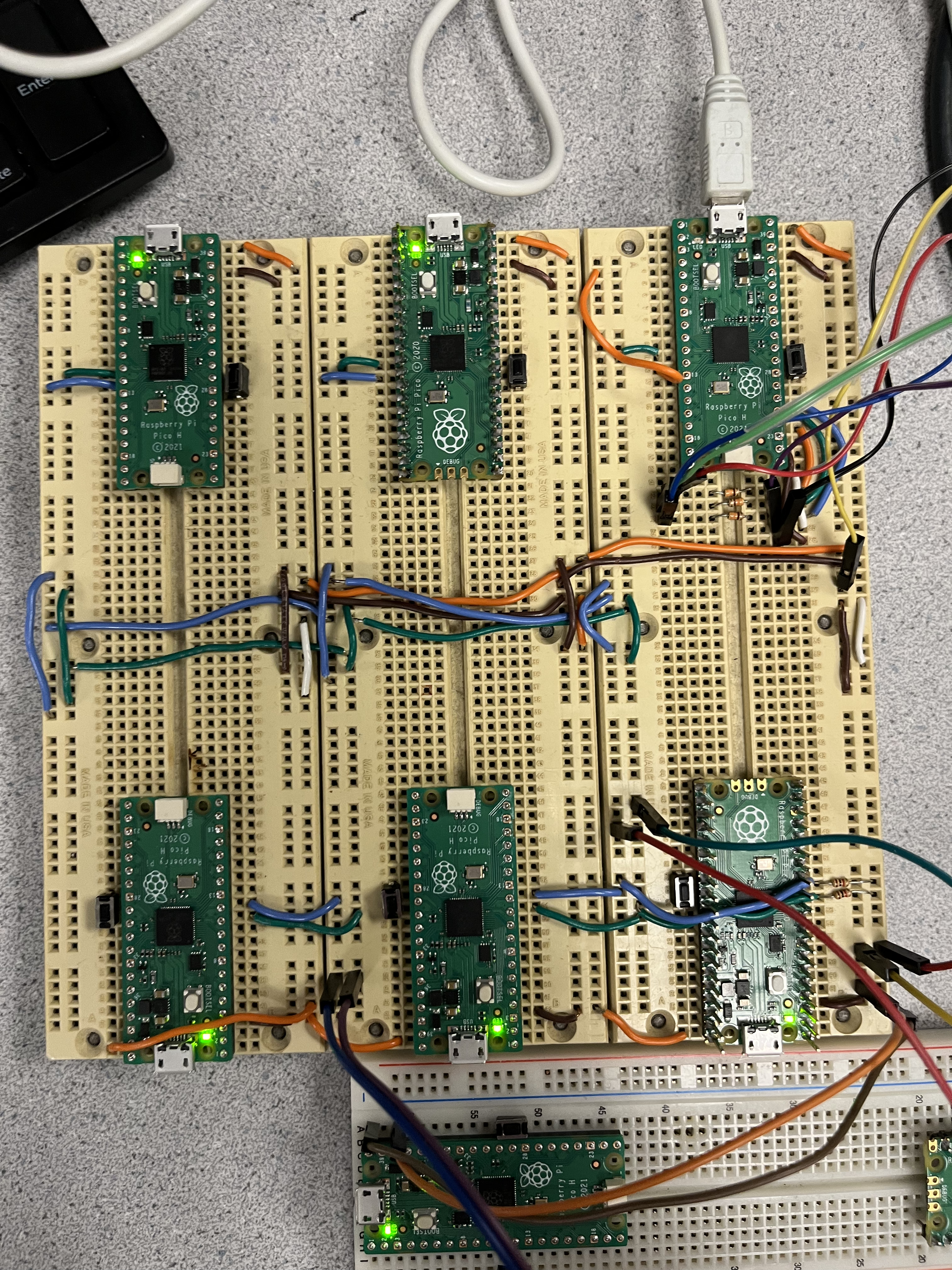
As far as hardware goes, the system we designed is relatively simple. Raspberry Pi Picos are all hooked up to the same power, ground, I2C SDA, and I2C SCL busses. The central projection Pico is also hooked up to the monitor via VGA for Mandelbrot display and to a laptop via UART for serial feedback. The serial monitor proved to be a useful tool when debugging, so we could read back how many Picos are detected on the network as well as other useful information.
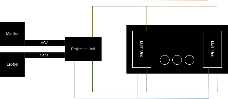
Once we had begun scaling up our system to include more than just a couple Picos, we realized that it would be necessary to better organize our hardware so units can be easily added and connected to buslines.
For our software design, we started with lightly modifying the Mandelbrot code from Hunter's examples. The set was computed with both cores using fixed point operations for faster computation.
We wrote two programs for this project, one for the main "projector" Pico and one for the rest of the "math" Picos. We wanted the projection Pico to detect the amount of math Picos available on startup, and for the math Picos to be assigned different ID numbers and also know the amount of Picos on the line. We designated the projection Pico to be an I2C peripheral and for the math Picos to be I2C masters. The Pico's I2C hardware is designed to handle multiple-master arbitration, so this was safe to do. We were able to get a hold of 8 Picos for this project, so we weren't able to test more than 7 on the line. We determined the number of Picos on the line and assigned IDs to each Pico with the following procedure on each type of Pico.
PROJECTOR
- For 2 seconds, each time a read is issued to it, send back a value (initially 1) and increment it.
- For each Pico that issued a read in step 2, detect a read and send back the total count of Picos.
- Issue a read for a Pico ID number.
- Wait 2 seconds.
- Issue a read for the total Pico amount.
An individual column of Pixels was divided between two cores, the two cores of the Pico assigned to that column. We had to be careful of the cores trying to use the I2C communication simultaneously, so we had to implement some kind of locking mechanism to block a core if both are trying to issue an I2C write at the same time. I experimented with hardware spinlocks, but I decided to use a pair of variables in the C code to act as semaphores. Before starting an I2C communication core, a core indicates that it's about to start a communication, but only if the other core hasn't started a communication. This prevented the cores from "interleaving" I2C communication data. Each computed pixel was sent to the projection in a 3 byte packet, where the x, y, and color info is packed into these bytes. Three bits for color, ten for the x-coordinate on the screen, and nine for the y-coordinate. We experimented with dead reckoning, where the projector Pico will keep track of how many packets have been received from each core, and draw the pixels out in a known pattern. The problem with this approach is that a few missed data packets will distort the result significantly, while a missed communication with coordinate information will only result in a few missed pixels. If the reliability issue was worked out, dead reckoning would have the advantage of decreasing the amount of data sent per pixel to one byte (three bits color, five bits for Pico ID for a maximum of 31 peripheral Picos).
During the computation of the Mandelbrot set, the projector Pico has a DMA channel set up to move received data from the I2C channel. Every time the Pico receives a write from one of the math Picos, the DMA channel moves the data from I2C to a variable in memory and initializes an interrupt routine to the processor (core 0). For the amount of data received, the CPU time spent in the interrupts was insignificant. (At an I2C max data rate of 1 MBPs, and 3 bytes per transaction, there's a maximum of 41,666 transactions per second. If an interrupt takes 100 cycles to execute, that's about 4 million cycles per second used to service these interrupts. This is small compared to the Pico's default 125 MHz clock).
Results
In the end, we were able to achieve a speedup of 3.86x with eight Picos connected compared to just a single Pico working on its own. As Picos were added to the network, computation time decreased at a rate that seemed to diminish as the number of Picos increased, suggesting that a horizontal asymptote exists for our system's performance. On the other hand, the total I2C transactions increased as the number of Picos increased in diminishing fashion, also appearing to approach some sort of horizontal asymptote.
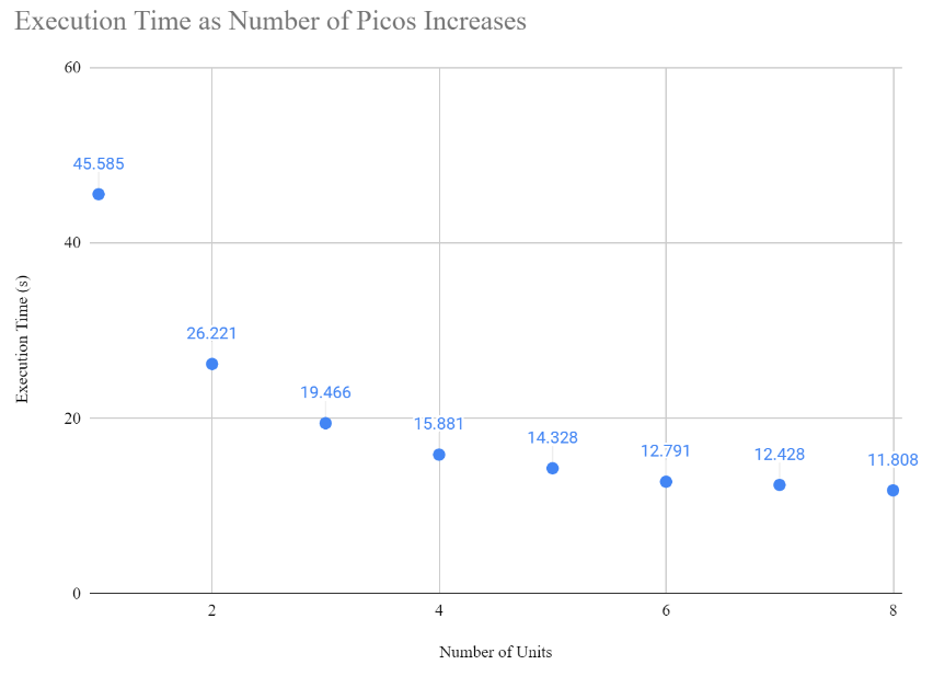
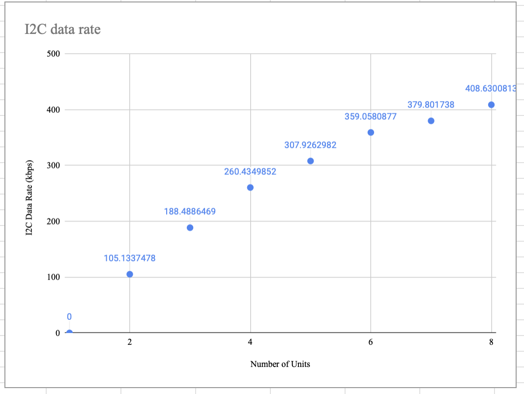
This suggests that communication is not the bottleneck of our design, because if it were then we would see a much more aggressive trend in the increase of I2C transactions. Because math units never communicate with one another, when a unit is added to the network the only additional communication that occurs is the setup for that new unit and the data transfer for the work no longer being done in the projection unit itself. Nonetheless, with many units the additional amount of communication required for data transfer when another unit is joined to the network is small. For example, with six units total the projection unit computes 106 columns, with seven units the projection unit is responsible for computing 91 columns, but with eight units it is responsible for 80 of them. Hence, as the number of units gets larger and larger, the amount of decrease in work the projection unit sees also decreases in diminishing fashion. Because of the diminishing nature of the increase in transactions, we believe that the limiting factor of our project is still the computation itself. It is also worth noting that while execution time varied slightly from trial to trial for a given number of Picos, the total number of I2C transactions was always the same.
Though it is a small detail, it is interesting to note that the execution time decrease going from six to seven units is only about 300 milliseconds, while the decrease going from seven to eight units is about 600 milliseconds. We believe that this illustrates the inequality of necessary computation effort between regions of the Mandelbrot set. In particular, we found that the region of the set highlighted with the green box below always took the longest to compute and display, regardless of the number of devices on the network:
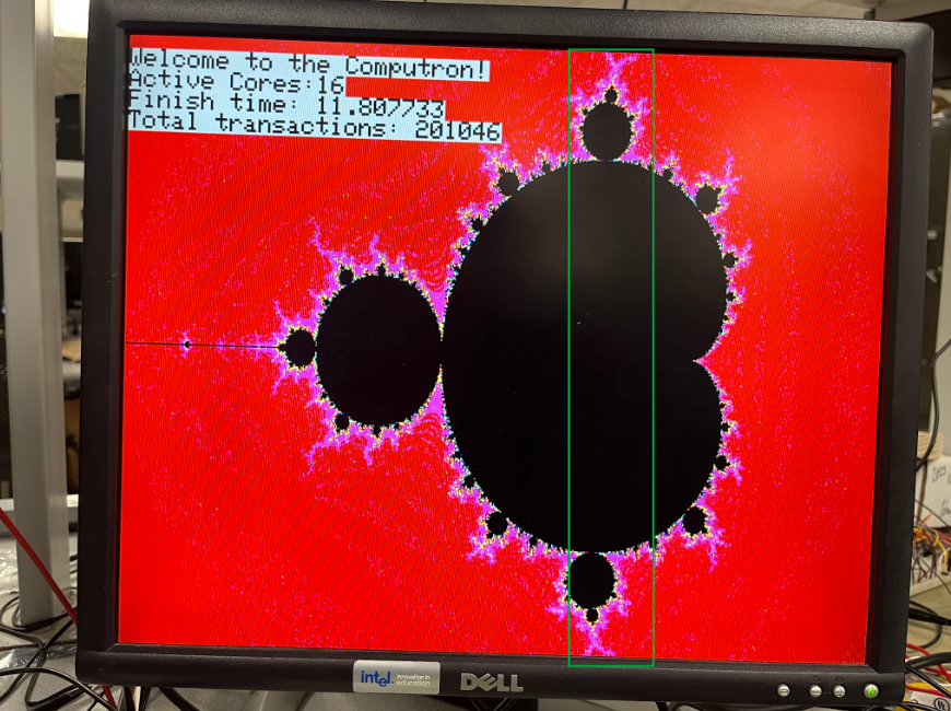
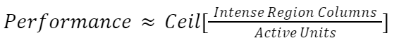
We believe that this region is so intense compared to the other parts of the screen to compute, that it computationally functions as a bottleneck. For instance, let us say that this region is 22 pixels wide. This means that for six Picos working together, four of them will have to compute four columns each from this region. When adding an additional Pico to have seven total, one would expect a significant speedup. However, in this case one of the Picos will still need to be responsible for four of these very computationally intensive columns. Only when eight Picos are in use does the maximum number of columns from this region to be computed by any single Pico decrease from four to three. This idea that this region coerces performance into not improving in a smooth, intuitive fashion is expressed by the following equation:
We also were able to achieve consistently lossless images of the Mandelbrot set by the end of our work on the project. This is significant, as our project is completely reliant on its visual outcome on the monitor. The only times at which the display glitches or fails are when not enough power is being supplied to our network, especially in the case of seven or eight Picos hooked up, or when the network is augmented after computation has already begun.
Furthermore, a prominent strength of our design is its usability. So long as a Pico is loaded with the code for the math units, it can be hooked up to the I2C line of the network and immediately integrate itself into the parallel computer. This is made possible by the setup logic explained earlier: because math units initiate communication with the projection unit, the number of Picos on the network is automatically variable and Pico IDs are automatically generated, meaning that the distribution of work is also automatically adjusted.
Conclusions
Conclusions This project is a great starting point for a future project where we may need more performance for an application that a single Pico can provide. The I2C communication we used was OK but there are many potential directions we can take to improve performance. In the future, we could try using SPI communication, structured in such a way to adjust for its single-master attribute, and CAN communication could increase communication speed in certain cases, like if multiple Picos had to share a data set. Our parallel computer using I2C communication between the Picos is an elegant solution to increasing computation speed of the Mandelbrot set. The 4x speedup is less than the 8x you'd expect from using eight times the hardware, but it's a solid basis for speeding up the mandelbrot set. The structure of using a single Pico for monitor operation can be useful for different projects as well. Perhaps the Pico could serve as a dedicated VGA display for a different microcontroller or small computer.
Appendix
Appendix A
The group approves this report for inclusion on the course website.
The group approves the video for inclusion on the course youtube channel.
Appendix B: Code
Link to a Github Repo containing our project's code: https://github.coecis.cornell.edu/ir93/ComputronParallelComputer.git
Appendix C: Responsibility Breakdown
Ignacio and Ryan were both together at all points developing the software and hardware. Ignacio handled a little more debugging of the system while Ryan worked on the hardware design and results section of this report.