ECE4760 Final Project: Digital Vocoder
Charlie Mueller - cmm478
Schuyler Seyram - ses398
Project Introduction
For our final project we built a digital vocoder allowing one to talk into a microphone and hear their transformed speech through a speaker. The main idea is to use human speech to modulate a synthesized carrier signal, which produces output speech that says what you are saying, but sounds nothing like you. For our project we chose and tested a handful of carrier signals, but spent most time using a sawtooth wave carrier because it produces the most electronic-sounding output. This made our vocoder sound more like an autotuner, which we found interesting because we wanted to produce output that sounded robotic. We were also able to allow the user to change the pitch of the transformed output manually, either raising it or lowering it. This was an important feature we wanted to add because we wanted our vocoder to be similar to an actual vocoder one could purchase, where a user can change the voice output at a bunch of different pitches and sounds, not just one. Overall, we finished with allowing the user to change which carrier signal was being used to synthesize the output, and the pitch of the output. This made our project more interactive, intuitive, easy to play with, and provided a wide range of ways one could disguise, transform, and change their voice.
High Level Design
Rationale and Sources
We initially spent a significant amount of time trying to decide what broad topic to develop our project in. The possibilities were overwhelming but we knew we wanted to do something with that involved data transfer or augmentation. Signal processing was a topic we had relatively little experience with, and we both were particularly fascinated by the bird chirp synthesis lab, so we decided to select an audio-based project. One of us was particularly interested in the range of human voice frequency we could capture and process with the Pico as compared to traditional laptops coupled with audio synthesis software. We also wanted our project to be something that people could actually use and make it as practical as possible, so for all these reasons we landed on a vocoder. We browsed past student projects and found that another group tried a vocoder in the past but couldn’t get it fully working due to the PIC32 processor not being able to run at a high enough frequency. We looked at the timing specs and observed that the RP2040 is clocked at over double a frequency from the PIC32 (125 MHz vs 50 MHz). With this gain in speed, along with overclocking and the multi core capabilities of the RP2040, we figured we could build a powerful vocoder that could fully transfer and manipulate speech.
Background Math
We took samples from the microphone input using the Pico’s ADC. We chose a sampling rate of 8kHz. So we took ]\ a continuous time signal (human speech), and made it discrete by taking samples at intervals of 125 microseconds. Given our discrete set of samples, we reconstructed a continuous time signal by outputting samples to the DAC. The Nyquist Rate tells us how fast we need to sample a signal with a given frequency to collect a set of samples that uniquely determines the original signal given our sampling rate. More precisely, if we try to sample a signal lower than its Nyquist Rate, then the set of samples we obtain could have been obtained by sampling other signals with different frequencies. This is called aliasing, and it would cause our continuous output signal to not capture the higher frequency components of the input signal. This is because these higher frequencies above the Nyquist Rate would be clipped down to lower frequencies that have the same samples at that sampling rate. We wanted to capture as much of human speech as possible, and even though speech has most of its frequency content around 100-400 Hz, we wanted to be able to capture up to 3.5 kHz which includes singing. The Nyquist Rate is two times the frequency of the input signal, so to uniquely capture signals up to 3.5 kHz, we needed to sample at a rate of at least 7 kHz. Our sampling rate of 8 kHz was then definitely sufficient to sample and reconstruct all the frequency content of the speech.
As described in the next section, the way a vocoder works is by sampling the speech and passing the samples through a series of bandpass filters each covering a different frequency range, allowing us to deconstruct the speech and carrier signals by their frequency content. We chose to use second order butterworth bandpass filters, which use the following filter equation:
This generates the current output y[n] given the current input x[n], past input x[n-2], past outputs y[n-2] and y[n-1], and coefficients b1, a2, and a3. The coefficients are calculated based on the cutoff frequencies of the bandpass filter. In our implementation we did not use arrays, which we will explain in the program design section.
The final part of the math we needed to consider was how to amplitude modulate the carrier signal. We pass the speech input and carrier signal through a set of bandpass filters, getting filtered samples of each. We need to impose the envelope of the filtered speech at each frequency onto the carrier sample. We accomplished this by first rectifying both filtered samples, and then low passing each to reduce noise. This gave us the envelope, or peak shape of both signals. Then, we could take the ratio of the speech envelope to the carrier envelope, and multiply this by the filtered carrier sample, forcing the carrier sample to take the same shape as the speech.
Logical Structure
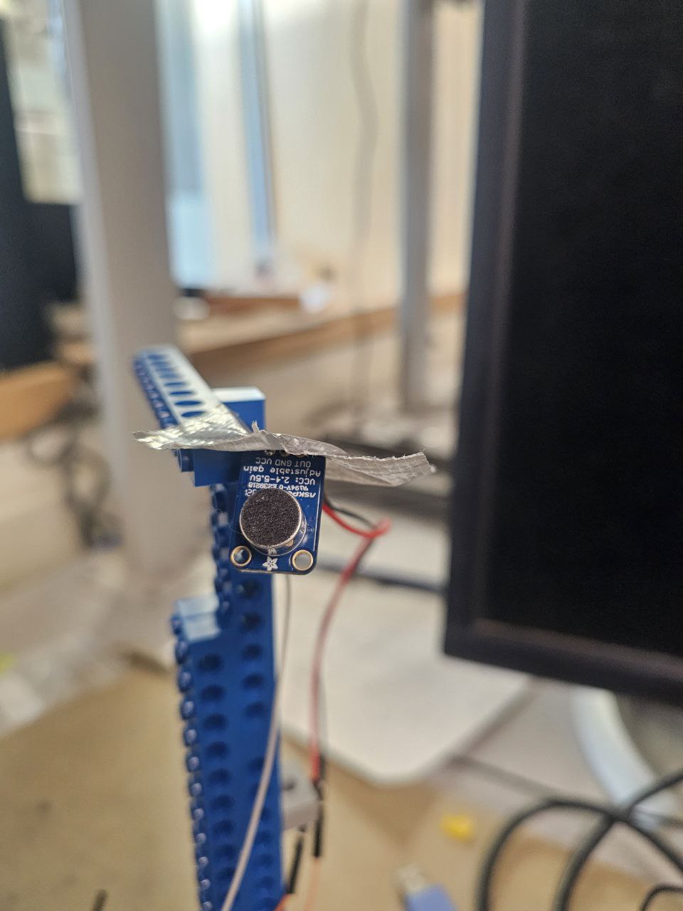
A vocoder works by analyzing the frequency content of signals. We used an AdaFruit microphone connected to the Pico’s ADC to get the speech. This microphone was powerful and simple to use as it required little setup. We sampled the ADC input at a rate of 8kHz to get our speech input. Each speech sample is then passed through a number of bandpass filters with different frequency ranges from 20 - 3999 Hz covering all of the frequencies we want to be able to capture. We also needed to pass carrier signal samples through the bandpass filters as well. However, one important fact that Hunter helped us with during the lab is that we needed the same number of carrier signal synthesizers as bandpass filters. For each filter, we send a carrier signal sample generated at the center frequency of that filter. So for 18 bandpass filters total, we synthesized 18 waves from the carrier signal, each one at the center frequency of the corresponding bandpass filter. So while the same speech sample is passed through all 18 bandpass filters, a separate carrier sample is passed through each filter. Then, the filtered carrier and speech sample are rectified and low-passed so we can find the peak of each with minimal noise. So for each frequency range (out of 18), we have the frequency content of the speech in that range, and a filtered carrier sample in that range. The ratio of the low-passed speech to low-passed carrier sample is then multiplied onto the filtered carrier sample, shaping the peak of the carrier sample for that frequency range to be the same as that of the speech’s frequency content in that range. Then, all 18 modulated carrier samples are summed up, and the resulting output is sent to the DAC.
Different carrier signals produce different-sounding outputs, so we created multiple carrier signals including: sawtooth wave, triangle wave, and white-noise. The user can use the keypad to select which carrier signal to use, and can also use the keypad to increase or decrease the pitch of the synthesized output. These instructions were displayed on the VGA screen to create a helpful interface for the user to know what they could do with the vocoder.
Program Design
ISR Organization
We set up an ISR on core 0 of the Pico to fire every 125 microseconds, or 8kHz. In the ISR routine we sampled a value from the ADC using adc_read(). We also kept a global variable containing the next output to be sent to the DAC. This is because we used a protothread to do all of the vocoder computations. We wanted output samples to be sent to the DAC immediately following sampling an input, rather than doing the computation inside of the ISR, which would send an output sample roughly 90 microseconds after taking an input sample. So, we used another global variable to indicate that there was an ADC sample ready to be used. The vocoder thread would wait until this variable was set, and when it was, the thread would then process the input sample using the filtering scheme mentioned above, and store the output in the global variable for the DAC output. The vocoder thread ran on core 0 as well. However, we still needed all of our computations to be less than 125 microseconds, otherwise the output sample from a given input wouldn’t be ready by the next time the interrupt fired, and we would be sending multiple copies of the same output. This had the effect of making the output speech delayed and a lot slower, which was a small problem we ran into.
Fixed Point Representation
The ADC and DAC both operate on 12 bit values. For the filter implementations, we needed at least 5 decimal bits of resolution as specified by Bruce in his DSP page, linked below and in the Appendix. He also helped us discover that 5 decimal bits corresponds to 16 fractional bits. It couldn’t hurt to get as much resolution as possible, so for our fixed point implementation we used 1 sign bit, 12 integer bits (to handle ADC/DAC data), and 19 fractional bits. We could use fixed point methods to then convert our ADC sample to fixed point for computation. To convert our output from fixed point to a 12-bit int for the DAC, we had to do something slightly more complicated because all of our computations handle negative values, but the DAC output cannot be negative. Instead of right-shifting by 19 we right shifted by 20, leaving a number between -2048 and 2048. We then added 2048 to shift the range from 0 to 4096, which is what the DAC accepts.
Carrier Signal Generation and Sampling
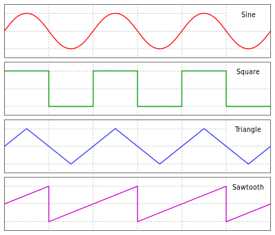
We generated carrier signals in main before the vocoder started running, so all of our carrier signals were arrays in memory. If we had more time, it would have been more beneficial to use direct digital synthesis to generate all of our carrier signals. We were only able to store 3 carrier signals in memory before running out of RAM. Each carrier signal was an array of length 8192 elements, we chose this length because we read how important it was for the carrier signals to be long enough to contain frequency content at a wide range of frequencies. We also normalized all carrier signals to contain values in the range of [0,1] to make sure they were all on the same scale. Each array represented one full period of the signal, so to generate samples at different frequencies we could use the size of the array to determine how many examples we needed to skip over at each iteration. Below are pictures of the final carrier signals we used.
Triangle:
Sawtooth:
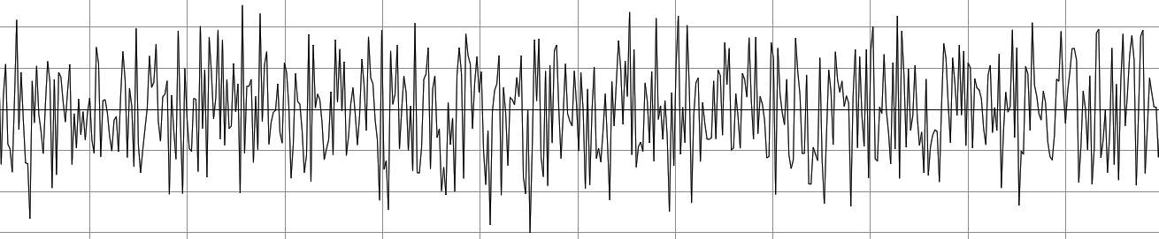
White Noise:
The triangle and sawtooth waves sounded very similar. We read about vocoder carrier selection online and saw that sawtooth was a popular choice because of its harsh, electronic sound. The white noise produces a very static-sounding output which is interesting to hear especially when a voice talks through it.
As mentioned above, since we had 18 bandpass filters we needed to use 18 synthesizers of the carrier signal. For each bandpass filter, we used an accumulator and incrementer to step through the carrier array at the center frequency of that filter. So, we had an array of 18 accumulators and an array of 18 incrementers. To calculate how much we needed to increment by we used the equation:

Then, in the vocoder thread we updated the accumulator for a filter by its increment and then took the modulo by the length of the carrier array to make sure our index is in bounds. We used a global variable to indicate what carrier signal we were currently using, so we knew which carrier array to grab a sample from using the accumulator.
Filtering
To implement the bandpass filters we used Bruce’s implementation of a second order Butterworth bandpass filter. Here is a link to his code file with the filter implementation, which worked very well and is a short and efficient implementation. However, each filter needs different coefficients based on the cutoff frequencies of the bandpass. To calculate those we used the Matlab function butter(), which we did for all 18 filters. We then kept the coefficients stored in a 3d array. The top-most array has 18 elements, the set of coefficients for each filter. Each of the 18 arrays has two elements: an array of A coefficients and an array of B coefficients. These coefficients are then passed into the filter function. We also had an array of 18 elements to keep track of the past x and y samples for each filter for use in the filter function.
Amplitude Modulation
To do amplitude modulation we low-passed the rectified filter speech and carrier samples first. To do this, we rectified using a simple absolute value function. We used a low-pass function written by a previous group trying to implement a vocoder. At first we did not low-pass because we weren’t sure it was necessary, but we struggled with the output being very noisy and sensitive to the surroundings, as there were many other people talking around us in the lab. We tried to figure out the characteristics of their low-pass function and what cutoff frequency they were trying to use but then settled on using their implementation to finish in time. Here is a link to their report webpage, which is where we found the lowpass function. Their report also helped us realize how to do amplitude modulation by multiplying the filtered carrier signal by the ratio of the low-passed speech to the low-passed carrier. A general structure of the main vocoder algorithm is:
for (i = 0; i < NUM_FILTERS; i++)
{
fix19 carrier_sample;
phase_accum_main_0[i] = (phase_accum_main_0[i] + phase_incr_main_0[i]) % carrier_table_size;
if(current_carrier == 1) {
carrier_sample = sawtooth_carrier_table[phase_accum_main_0[i]];
} else if(current_carrier == 2) {
carrier_sample = whitenoise_carrier_table[phase_accum_main_0[i]];
} else if(current_carrier == 3) {
carrier_sample = triangle_carrier_table[phase_accum_main_0[i]];
}
fix19 sample = bandpassFilter(adcSample, coefficients[i][0][0], coefficients[i][1][1], coefficients[i][1][2], pastSpeechN-2[i], pastSpeechN-1[i], pastSpeechOutputN-2[i], pastSpeechOutputN-1[i]);
fix19 amplifiedSample = lowpass(abs(sample));
fix21 filteredSig = bandpassFilter(carrierSample, coefficients[i][0][0], coefficients[i][1][1], coefficients[i][1][2], pastCarrierN-2[i], pastCarrierN-1[i], pastCarrierOutputN-2[i], pastCarrierOutputN-1[i]);
fix21 amplifiedSig = lowpass(abs(filteredSig));
DAC_output += amplifiedSig != 0 ? multfix19(filteredSig, divfix(amplifiedSample, amplifiedSig)) : 0;
}
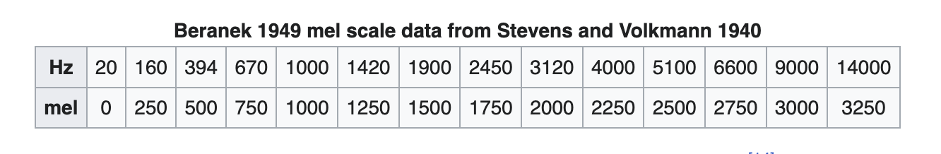
We started off with only 8 filters, distributed according to the Mel scale:
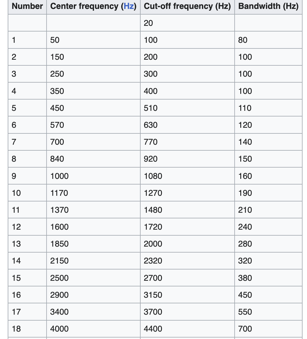
but quickly realized we were only using a small fraction of the time we had to compute. So, to increase the amount of speech data we could capture, we switched to the Bark scale, which used 16 filters for the same range of up to 3120 Hz for which the Mel scale only used 8. A diagram is below. The 18 ranges shown in the Bark scale were the 18 bandpass filters we ended up using. This improved the performance of our vocoder notably. It is also important to note that these acoustic scales select frequency ranges that appear equidistant in pitch or “loudness” to listeners.
Bark Scale:
Keypad Debouncing and VGA
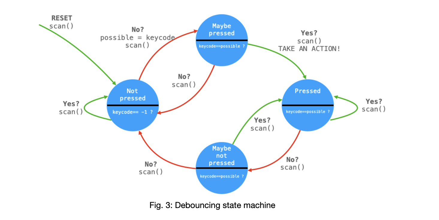
We used one thread to take in keypad input and write to the VGA screen. This thread ran entirely on core 1, taking advantage of the Pico’s multi core capabilities. Core 0 was responsible for all of the vocoder computation and I/O, while core 1 was responsible for taking I/O from the user keypad and displaying instructions on the VGA. This way, on core 0 we had the full 125 microseconds in between ISR’s to only do vocoder computation and implement as many filters as we could. In the keypad thread 1, we used a debouncing FSM from lab 1 to determine if a user was actually selecting a button. Here is the FSM diagram:
This image is taken from the lab 1 keypad webpage created by Hunter (link)
The instructions we displayed on the VGA screen where:
-Press 1 to select a sawtooth carrier wave
-Press 2 to select a white noise carrier wave
-Press 3 to select a triangle carrier wave
-Press 4 to increase pitch
-Press 5 to decrease pitch
Thus, if we detected that some action was taken (user pressed a button) from the FSM, if they changed the carrier wave we changed the global variable indicating the current carrier wave. Increasing the pitch corresponds to raising the frequencies that the 18 carrier wave synthesizers are taken from. This was discussed earlier, when we mentioned that for each filter, we generate a carrier sample from the carrier array at the center frequency of that filter’s range. So, to increase the pitch we increased the frequency we were using to generate each carrier sample for each filter. To decrease pitch, we just had to decrease these center frequencies. Since the frequency ranges of the filters are not all the same length, we calculated 10 percent of the width of each range, and used that as an increment/decrement amount. This allowed the user to increase or decrease the pitch many times consecutively to give them more of a finer-grained control over the system.
Hardware Design
This project was really focused on the application of the Raspberry Pi Pico to function as an embedded system with little or no help from external components. As a result, our hardware setup was simplified. Our filters were all software based rather than hardware. As a result, we only used these components:
I. Raspberry Pi Pico
Ii. Copper wire
III. Microphone
IV. VGA monitor
V. Numeric Keypad
VI. DAC(Digital to Analog Converter)
VII. Audio Jack
VIII. 330 Ohm resistors for keypad and the VGA connection
The vocoder sound synthesis pipeline is as follows:
Input of speech through mic -> Raspberry Pi ADC -> Software filters-> Carrier waves-> GPIO Output to DAC-> DAC-> Audio Jack-> Speaker.
In parallel to this pipeline is a keypad and a VGA output
The microphone consists of 3 terminals: VCC, GND and Output. The GND is connected to the GND of the Pico and is powered through the 3.3V output of the Pico. The output of the microphone is then connected to one of the Pi GPIOs.
The output of the Pico after signal processing is sent from the Pico via GPIO to the ADC(Analog to Digital Converter) via SPI protocol. The DAC draws power from the Pico through VDD and VSS is connected to ground. The CS SDK SDI and LDAC are all connected to the Pico. The DAC has 2 outputs, Vout A and B, one for each channel, ie. left and right. One of them is then connected to one of the audio jack pins through the breadboard. The audio jack has 3 pins,one for ground and 2 for left and right inputs. The audio jack then transmits to the speaker which emits the warbled electronic voice. The SPI configuration for the DAC is as follows:
CS -> GPIO 5
SCK -> GPIO 6
MOSI -> GPIO 7
LDAC -> GPIO 8
VDD -> 3.3V Out
VSS -> GND
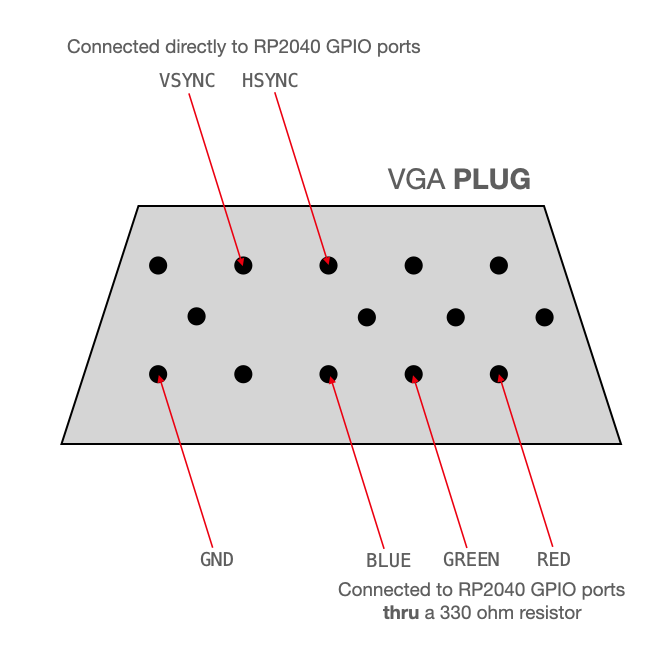
VGA Connection:
We modeled our VGA connections after the example received in lab 2:
The VGA is connected as follows:
GPIO 16 ---> VGA Hsync
GPIO 17 ---> VGA Vsync
GPIO 18 ---> 330 ohm resistor ---> VGA Red
GPIO 19 ---> 330 ohm resistor ---> VGA Green
GPIO 20 ---> 330 ohm resistor ---> VGA Blue
RP2040 GND ---> VGA GND
It’s a bit intuitive as to why we have a GPIO for RGB. Colors for screens are formed by a mix of red and blue, with the Pi outputting voltage for each corresponding color. One can say the range of 0-0.7V corresponds to 0-255. However , the VGA needs some guidance to refresh or move throughout the screen, which is where VSYNC and HSYNC come in. VSYNC sends the signal to start a new frame on the screen while HSYNC tells the screen to move to a new row of pixels.
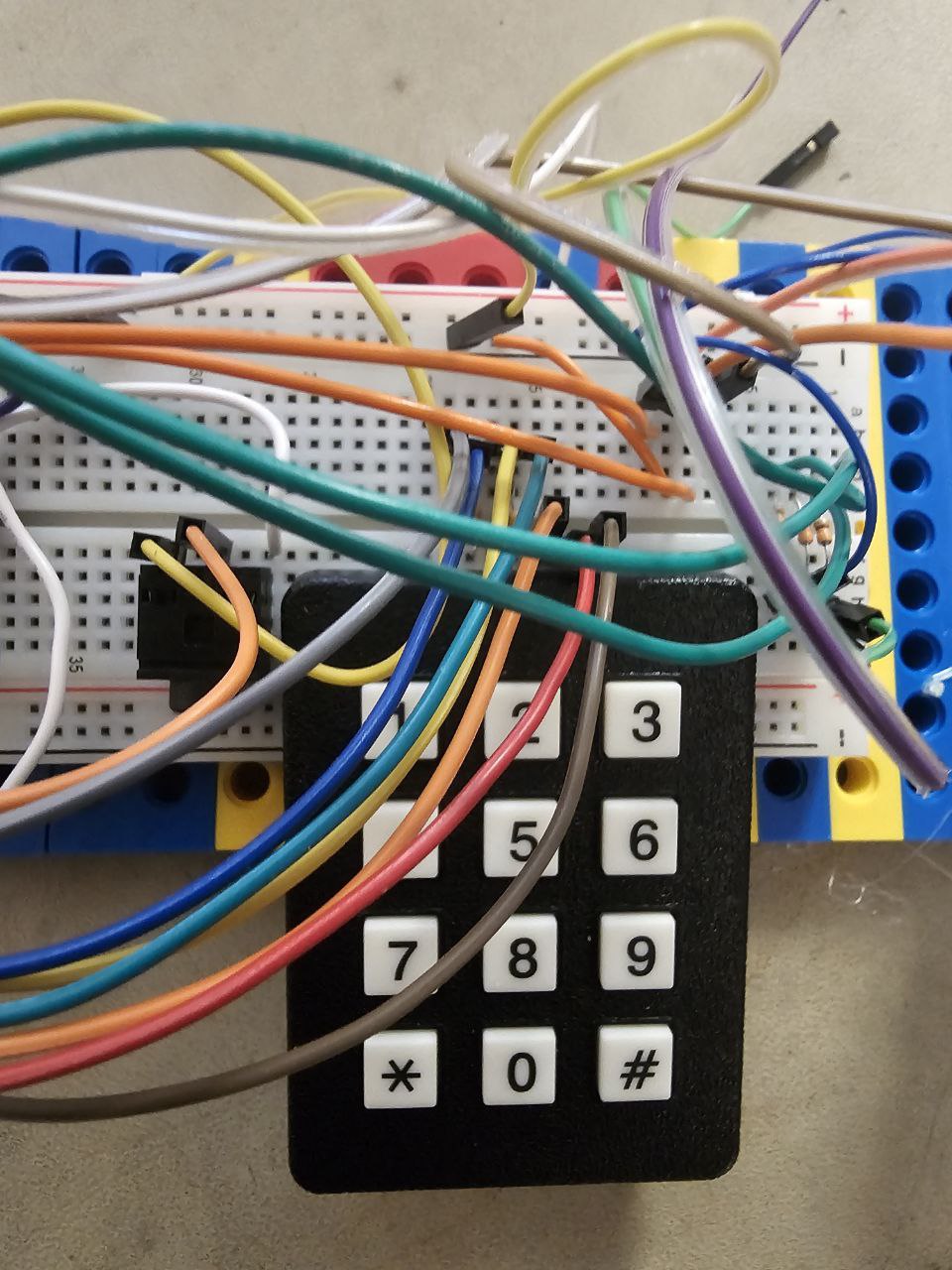
Keypad
The keypad has 4 rows and 3 columns. It uses 7 GPIOs to determine input. ie(GPIO 9-15)
Simply put, the keypad is scanned and GPIO input from all 7 pins are taken and masked. The resulting 7 bit number represents one of the pins on the keypad and so can tell which key is pressed based on which 2 GPIO pins are high.
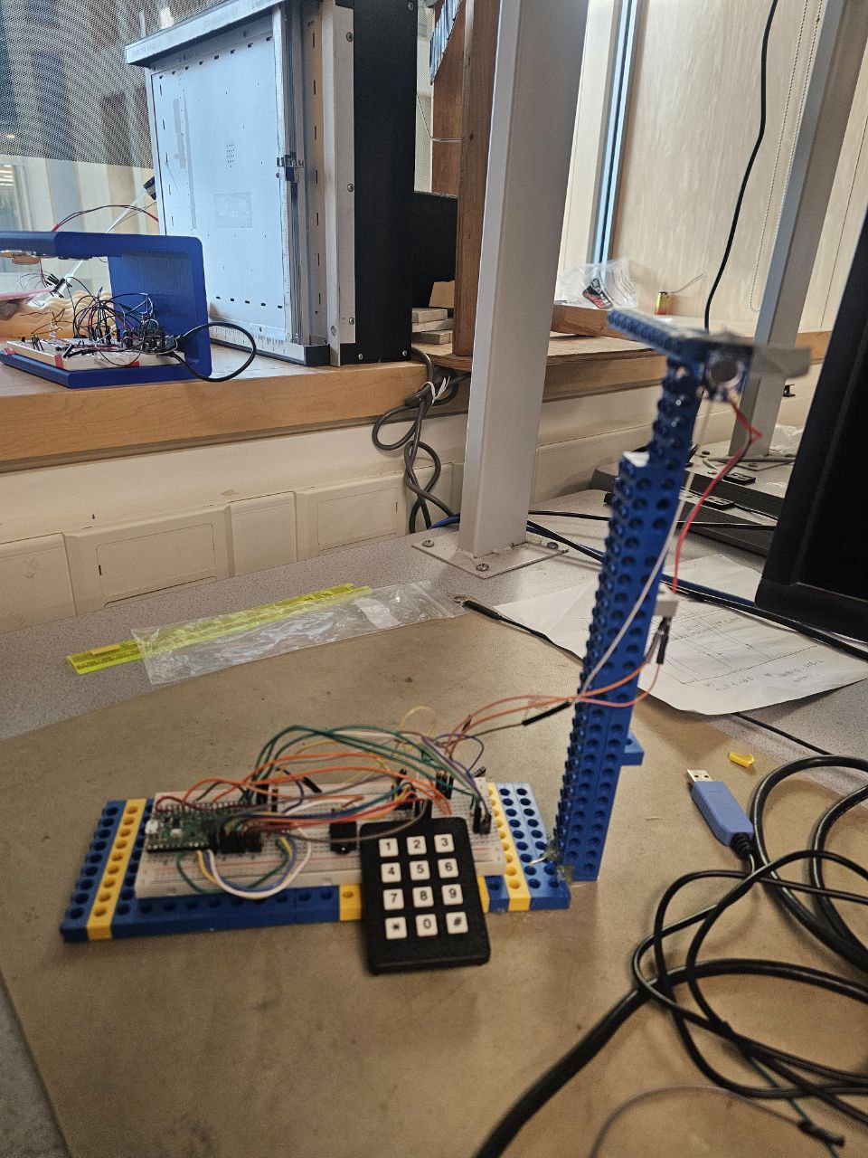
Full Setup(minus monitor screen)
Results
As mentioned earlier, we started off with less filters than we have now. The end result was an 18 filter vocoder with a range from 0-4kHz. Each filter had its corresponding synthesizer with a center frequency based on the range of the bandpass filter. Using keypad input the synthesizer center frequencies were increased or lowered, changing the pitch. Carrier waves could also be swapped and sound quality was pretty good. In our demo, we displayed the time needed to generate each DAC sample (all of the vocoder computation). In total we consistently needed around 96 microseconds. Our upper bound was 125 microseconds, so we still had some considerable time left over. If we had more time to work on the project we could have utilized this time better, and maybe even overclocked the Pico to get more time. We also could have improved the portability of the design with more time. This includes making a more solid stand for the microphone. We could have hidden the circuitry from the user and only made the microphone and keypad available to them, which would have been a lot cleaner and easy to understand for the user.
Conclusion
This project met our expectations and widened our scope when it came to audio synthesis. It led us to understand how sound is manipulated and processed digitally and taught us how to process sound: ie, it’s best to deal with ranges of frequencies rather than the whole spectrum of frequencies at a go.
Further Theoretical improvements
Given more time, our goal was to add more carrier waves and synthesize higher frequencies till the vocoder could manipulate sound as a result of humans singing. One limitation faced was memory. We faced an insufficient RAM error in trying to add another carrier wave table. The solution to this would have been to install some kind of readily available external memory module such as FRAM. Also based on our 8kHz sampling , our limit was 4KHz. Attempting a higher range of frequencies could have been achieved by overclocking the processor. Furthermore the incorporation of DDS(Direct Digital Synthesis Would have saved us more RAM.)
Appendix A
The group approves this report for inclusion on the course website.
The group approves the video for inclusion on the course youtube channel.
Appendix B
List of tasks carried out by each group member.
Charlie: ISR set-up, ADC set-up, DAC set-up, bandpass filters and amplitude modulation
Schuyler: Worked on carrier signal definition and synthesis, keypad debouncing, VGA set-up and display
Appendix C
References:
Bruce’s DSP Page: [1]
Bruce’s Butterworth Bandpass Implementation: [2]
Vocoder Report, by Jonathan Gao and Nicole Lin: [3]
Bark Scale: [4]
Mel Scale: [5]
Pi Pico Datasheet: [6]
Lab 1 Page for Keypad: [7]
Lab 2 Page for VGA setup: [8]
Appendix D
Link to the Github Repo: https://github.com/schuylerseyram/4760-vocoder.git