ECE 4760 Final Project: The Interactive Lightsaber

Berk Gokmen (bg372) and Justin Green (jtg239)

Our project is a 24-bit RGB LED illuminated lightsaber that reacts to surrounding sound and detects vowels.

Demo Video

Introduction

In Star Wars, each character has a fixed lightsaber color. Despite being two big Star Wars fans, we wanted to change the fixed notion of lightsabers by creating one that would enable its users to have a lightsaber that could be more than one color. So, using a microphone, RP2040, and an addressable LED strip, we created an interactive lightsaber that changes based on audio input.

The first mode, disco mode, changes the color of the lightsaber based on the frequency and intensity content of the surrounding sound. This was done through an FFT to gather frequency and intensity, which were then mapped to HSV, where hue was determined based on the frequency and intensity configured the saturation and value. Later, HSV was converted to RGB to be displayed on the lightsaber.

The second mode, vowel detection mode, changes the color of the lightsaber to red if the user says "EE" and to blue if the user says "AH." This was done through the use of cepstral analysis, which involves computing the FFT of the log-power spectrum, lowpassing, and achieving a smoothed power spectrum through an inverse. This enables extracting the formant frequencies of the input sound, which we then compare with the formant frequencies with EE and AH to determine if there is a match.

High Level Design

Rationale of Our Project:

The original vision of our project was to build an interactive lightsaber with two modes: Disco mode and Character mode. Disco Mode changes the color of the lightsaber based on the surrounding sound frequency and loudness. This mode was implemented in the final design. Character mode, on the other hand, changes the color of the lightsaber to the specified character's lightsaber color. For example, saying "Darth Vader" would change the lightsaber's color to red. However, this mode was too ambitious for a 5-week project; therefore, we decided to create a more achievable "vowel recognition mode" instead, which changes the color of the lightsaber based on the user saying EE or AH.

Disco Mode:

For this mode, we want the lightsaber to change color based on the input from the microphone. To do so, we would need a function that takes in the frequency and intensity content of the surrounding sound and converts it to an LED color.

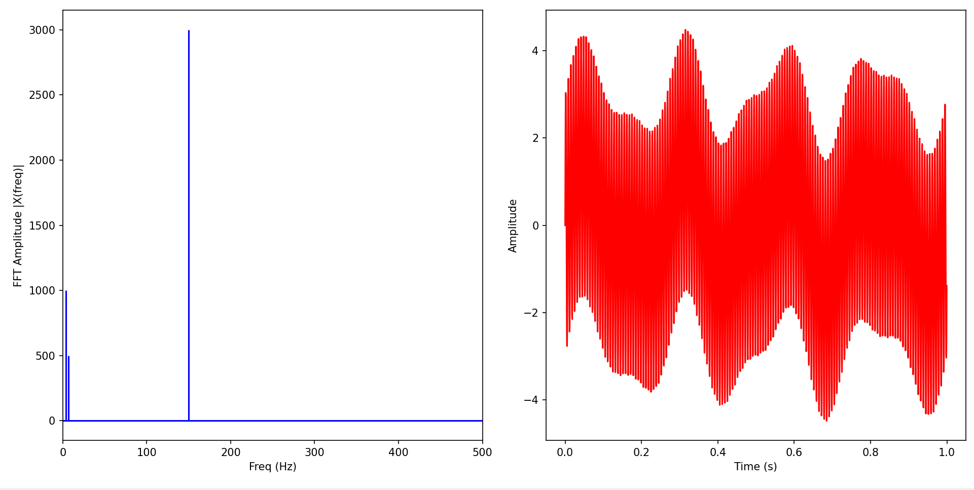
We decided that the input frequency to the LED function should be the most intense frequency in the surrounding sound, and the input intensity to the function should be the intensity of the most apparent frequency. The simplest method to find such frequency and intensity is using an FFT. The figure below illustrates a random signal and its FFT.

Figure 1. Random signal (on the right) and it’s FFT (on the left)

In this example, the most apparent frequency is at 150 Hz with an intensity of 3,000. This is clearly visible in the FFT. Therefore, through this method, we can easily extract the maximum intensity and frequency of the signal.

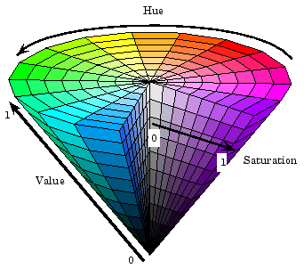
After finding the frequency and intensity content of the input signal, we wanted to convert these to RGB in a simple, linear function. However, RGB has three distinct color components, making it difficult to map from frequency and intensity to color. Consequently, rather than converting it directly to RGB, we decided to convert frequency and intensity to HSV first and then convert HSV to RGB. HSV also has three components: hue, saturation, and value. Hue ranges from 0 to 360 degrees, and saturation and value range from 0 to 1. The image below shows how each parameter varies the resulting color:

Figure 2. Illustration of how hue, value, and saturation changes output color. Source: Appendix B, 9

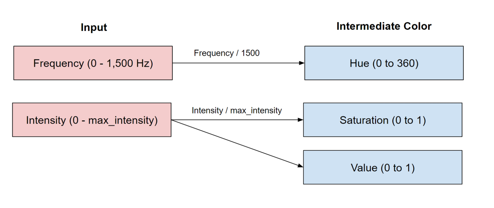
As seen by the figure above, the hue controls the base color, while intensity and saturation control the purity and brightness, respectively. As a result, unlike RGB where three distinct channels control the color, in HSV, only the hue impacts the base color, so we can easily create a linear mapping from frequency to hue. Then, we can map intensity to saturation and value. As a result, given a frequency (0 to 1,500 Hz), we scale the frequency to the hue spectrum (from 0 to 360 degrees), and given an intensity (0 to max_intensity), we scale the intensity to the saturation and value spectrum (0 to 1). The diagram below illustrates this transformation:

Figure 3. Transformation of input frequency and intensity to HSV

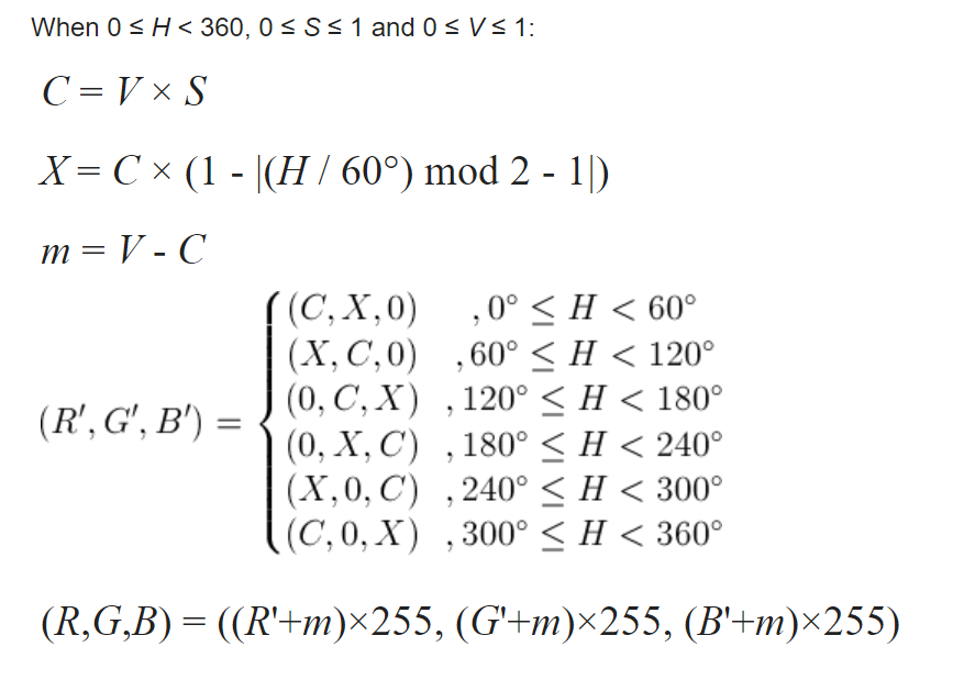
After the frequency and intensity is linearly mapped to HSV, the last step of the disco mode is to convert HSV to RGB, which is a commonly used formula illustrated below:

Figure 4. Formula for HSV to RGB. Source: Appendix B, 10

To summarize this process, we first obtain the most intense frequency and its intensity using an FFT. Then, we linearly map the frequency and intensity to HSV by mapping frequency to hue and intensity to saturation and value. Finally, since the LED accepts RGB, we convert HSV to RGB.

Vowel Recognition Mode:

In order to achieve vowel recognition for recognizing the difference between EE and AH sounds (or any other vowel), we need to extract a set of frequencies called “formant frequencies,” which represent the acoustic resonance at particular frequencies. This method works perfectly for our vowel recognition functionality because each vowel sound has a set of unique formant frequencies, illustrated in the table below:

Figure 5. Set of formant frequencies for several vowels. Source: Appendix B, 11

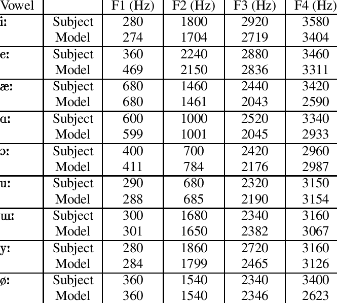
For our case, we are interested in the frequencies of the EE and AH sounds. According to the source corpus (see Appendix B, 12), the table below shows the expected formant frequencies of the EE and AH sounds:

Table of Formant Frequencies for EE and AH sounds

As a result, if we can successfully extract the input signal's formant frequencies, we can easily compare the extracted frequencies with the expected ones of EE and AH and pick the one that matches it the best.

To classify a sound as EE or AH, first plan to use a fixed range to see if frequencies fall in a given range. Then, we plan to use a fixed range and L1 distance as it is computationally light and an easy way to compare how close a set of three formant frequencies corresponds to the set of expected ones. The formula below shows how L1 computation is done:

An important note about formant frequencies is how much they differ from person to person (especially male to female). As a result, we plan to make the classification somewhat loose to account for frequency changes depending on the person. Loose classification may cause misclassification; we plan to test this after completing the system.

As mentioned earlier, the success of this functionality relies heavily on extracting the formant frequencies in an accurate and timely manner. To do so, we plan to use a method named cepstral analysis, which involves six steps:

1. Pre-emphasis: Boosts the higher frequency components of the input.
2. Window: Apply cos window to add periodicity to input.
3. Compute log power spectrum by taking the FFT, taking the magnitude of the FFT, and taking the log2 of the magnitude.
4. Convert to cepstrum: Take the FFT of the log power spectrum.
5. Truncate/lowpass: Smoothens final output and gets rid of fast changes in the cepstrum.
6. Convert back to the power spectrum by taking the inverse FFT.

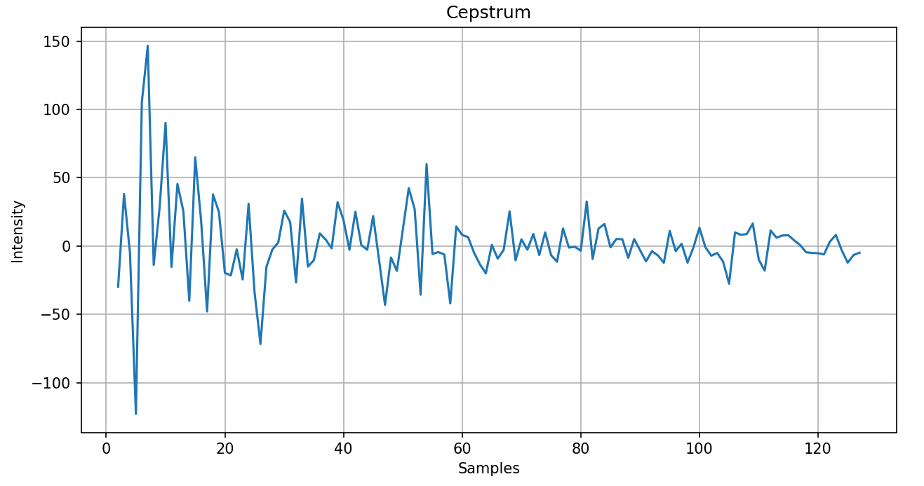
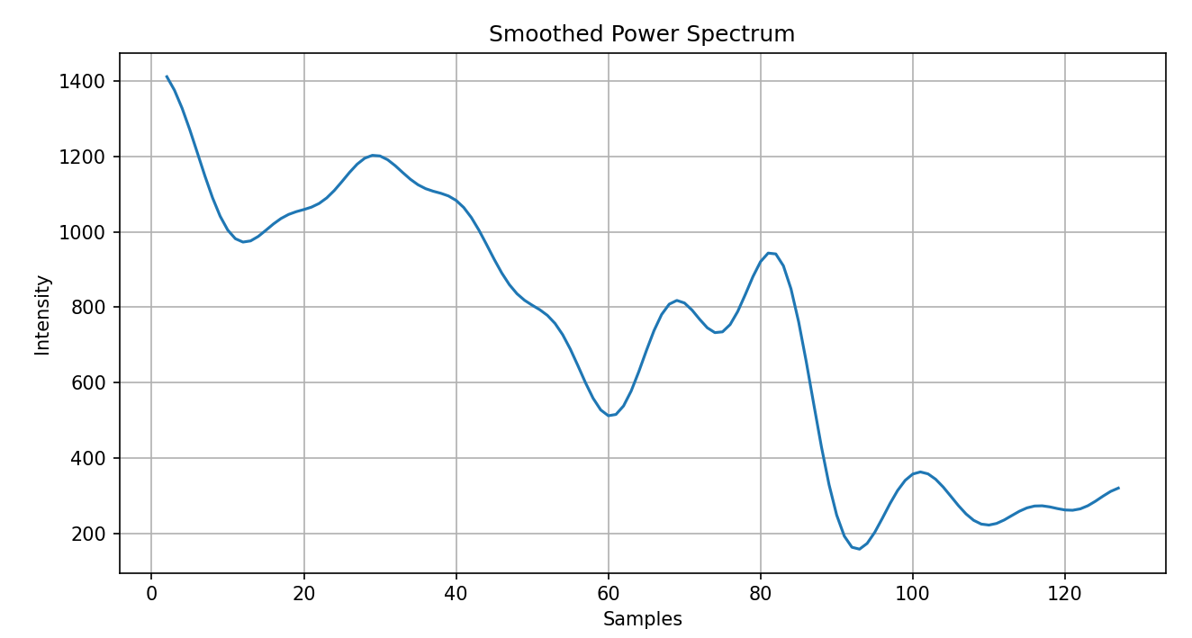
The figures below demonstrate the cepstrum and the smoothed power spectrum for a random signal:

Figure 6. Cepstrum of a random signal

Figure 7. Smoothed power spectrum of a random signal

As seen from the above graphs, the cepstrum appears sporadic and hard to analyze, while the smoothed power spectrum appears less daunting and visually more appealing, which is the primary purpose of creating this smoothed spectrum. The x-axis in both graphs corresponds to the sample. For example, the above graphs have 128 samples, and if they can detect frequencies from 0 to 4,000 Hz, each sample would correspond to a 4,000 Hz / 128 = 31.25 Hz window. Thus, if a peak was detected at sample 10, there is a formant frequency of around 312.5 Hz. Thus, to extract the three formant frequencies, we would find three peaks and which frequency window they correspond to.

To summarize the entire vowel recognition process, we first use the six steps above to get the smoothed power spectrum of the signal. Then, we pick the first three peaks above a certain noise level determined based on experiments and extract the frequencies of these peaks (which correspond to the formant frequencies). Then, we compute the L1 distances of these frequencies with the expected formant frequencies of EE and AH sounds. If the distance meets the criteria of the classification, then it is recognized as an EE or AH sound.

Software and Hardware Trade Offs:

The two leading hardware trade-offs are the microphone quality and the quality of the onboard ADC on the RP2040. As the microphone gets more expensive, the quality of the acquired input signal improves, enhancing the output of the FFT and the power spectrum. However, when we ran the example FFT code, the microphone from the lab did a sufficient job of displaying the correct FFT, so we decided to use the cheaper microphone. Another hardware trade-off is the onboard ADC, which impacts how frequently we can sample data. Due to the space constraints of the lightsaber, we did not want to use an external ADC, which worked perfectly with a sample rate of 48 MHz.

The leading software trade-off is the one between time resolution and frequency resolution. Decreasing the number of collected samples improves time resolution as fewer samples are collected per time frame; however, now, each sample corresponds to a larger frequency window, which reduces the frequency resolution. Increasing the number of samples has the opposite effect. Similarly, increasing the sample rate necessitates a decrease in the number of samples collected as well since the sample rate of the ADC is fixed.

Existing Patents/Copyrights:

There are no patent issues we need to worry about for this project. There is Disney’s lightsaber patent; however, this patent is for a real lightsaber where the blade is extended using illuminated light, rather than one being used with LEDs. Additionally, it has no audio detection features. However, the entirety of our mechanical design is adapted from the Star Wars Store’s lightsaber (Appendix B, 14), since we built the lightsaber by purchasing their toy and modifying it for our purposes.

Program/Hardware Design

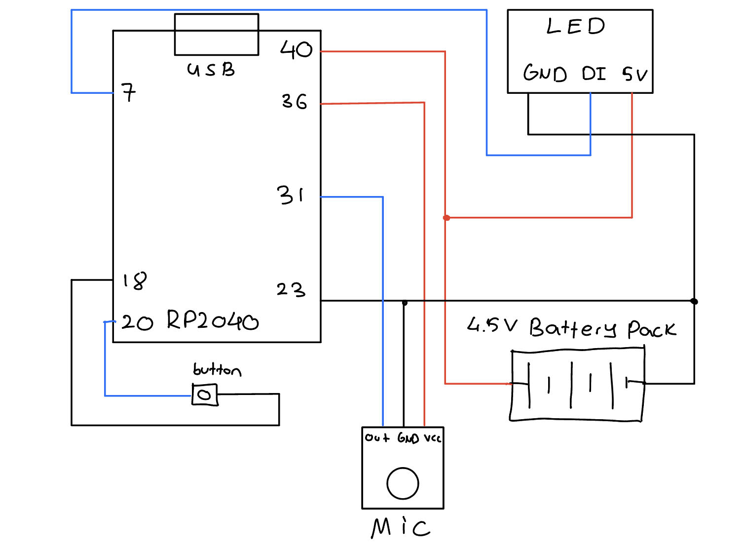
Microphone

We used a max 4466 MIC Amp as our microphone. The microphone has adjustable gain which we utilized by twisting the knob for potentiometer counter clockwise. The sensor is powered to 5V.

To send data to the Pico we used the on board ADC. The only hardware required was a connection to Pico GPIO 26 from the out pin on the microphone. This enabled us to utilize ADC channel 0 on the Pico to handle the data transfer. All that was required from our department on the software was to enable the ADC pin, select the correct channel and set up the ADC FIFO shown below:

FFT

A key aspect to our program was taking an FFT of the audio sampling data to allow us to actually be able to use the data. For our disco mode, we only needed to take a singular FFT to determine the frequencies and associated intensities to use. For vowel recognition we take three separate FFT’s as described in the high-level design section. Thus, the FFT was integral in the operation of our project. We utilize the FFT algorithm adopted by Hunter Adams (Appendix B, 15).

Although the cepstral analysis requires the use of an inverse-FFT to get back to the power spectrum, we do this by using a regular FFT. This is because taking the FFT of an FFT brings the data back to the same domain as taking its inverse. The only difference between the two processes is the scaling factor, which in our case, is not relevant as we only care about the relevant intensity of frequencies.

Audio to HSV

To convert the audio to HSV data was very simple. We just set the saturation and value components equal to the passed in intensity and normalized the intensity to a range of [0.1,1]. Then we set the hue value to the peak frequency normalized to a range of [0,360]. The 0.1 allowed the LEDs to not be empty.

HSV to RGB

Then we converted our HSV values to RGB values using Bruce Land’s algorithm (Appendix B, 7). The algorithm is displayed below. We called this function from the audio to HSV function with the calculated hue, saturation, and value. This process was done exactly as described in the high level design section. See Appendix B, 11 for HSV to RGB implementation details.

RGB to LED

Once we calculated our RGB value, we could finally illuminate our LEDs. We used WS2812B individually addressable LEDs. Raspberry Pi has a documented library ws2812.pio.h (See Appendix B, 13). The library utilizes Pico's PIO state machines. They run on about 3.5 to 5 V. The LED strip had three hardware connections: power, ground, and a GPIO pin to use for the PIO state machines as an input.

To start programming the LEDs, we programmed to the PIO which did as shown below. We also need to initialize the ws2812_program from pico-examples (Appendix B, 13).

To write to a singular LED, we utilized a function put_pixel  which takes in a 32 bit RGB value, and puts it off the PIO to write to the LEDs. Two important facts to consider were in our call to the PIO: pio_sm_put_blocking(pio1, 0, pixel_grb << 8u).   We left shift the rgb value 8 bits. Since the LEDs are 24 bit color, the least significant 8 bits have no effect on the output. Secondly in our ws2812_program_init  call, the last parameter IS_RGBW , proved to be important as when we initialized the parameter to be true, the LED did not shift the correct value which resulted in inconsistent color patterns. To elaborate further, when set high, the PIO checks 32 bits before moving onto the next 32. So after the first iteration where there are 24 bits used, the next iterations 8 most significant bits are included in the previous 24. The next iteration, the PIO looks at the remaining 16 bits with the first 16 bits of the following iteration. Therefore, everything became a mess of color. So the parameter was set false. The LEDs shift through the chain until there are none left, so to write to a set number of LEDs you must iterate through a loop number of LEDs and call put_pixel .

Initially we turned off all the LEDs by just writing nothing to them at the start.

Cepstral Analysis and Classification

Most of the cepstral analysis has been described already, but to emphasize, the implementation was extremely difficult due to a large number of moving parts. We used the VGA screen to incrementally work through the implementation by plotting different graphs and making sure we had the correct behavior.

For our classification, we took the formant frequencies of two sounds, AH and EE, and determined a range of the first and second frequencies that fit our own inputs. We looked at 7 point peaks of the cepstrum shown below

The zero index of the peak array corresponds to the first formant frequency, the one index corresponds to the second formant frequency and the two index corresponds to the third formant frequency. Once we calculated these values we checked if the first and second formant frequencies were in the AH or EE ranges (described more in the results section) and if so we would change the LEDs to the correlated color. If the ranges weren’t detected, we used the L1 distances as a backup classification. AH made the color blue and EE made the color red.

Mode Switching

We used an external button to switch modes. From a hardware perspective, we needed a GPIO pin (GPIO 15) and ground for the button. We just needed to initialize the GPIO pin, set the direction as an input, and add a pull up resistor.

In terms of changing states, we just toggle the mode variable if a button press is detected.

Mechanical and Electrical Assembly

Most of the connections were elaborated, but the only additional piece of important information is that we powered the system through 3 AA batteries, which was about 4.2 - 4.4 V. Our mechanical design was adapted from a Star Wars Store lightsaber (See Appendix B, 14). We removed the outer layer to fit the LEDs, and put the Pico inside of the saber. The circuit was soldered onto a protoboard  on the outside of the saber with the microphone taped onto the outside of the saber. The LEDs were attached to a 3/8 in by 3/16 in by 15 ft foam weatherstrip seal on both sides to have a more uniform color display. The battery pack additionally did not fit inside the saber.

Here is a holistic circuit diagram of what we created as well as the image of the final assembly.

Figure 8. Lightsaber electrical circuit schematic

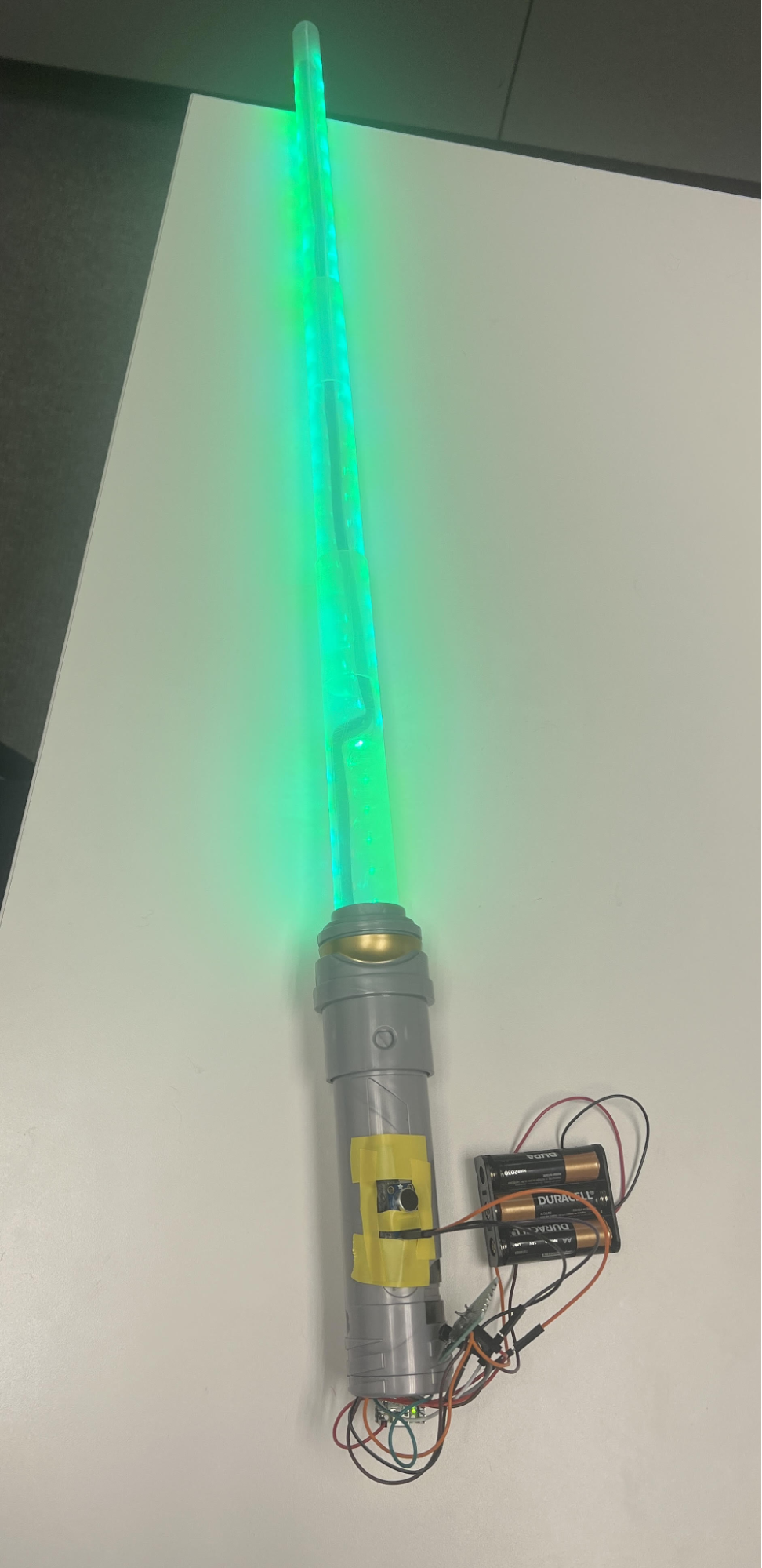
Figure 9. Picture of the final assembly

Results of the design

Disco Mode Results

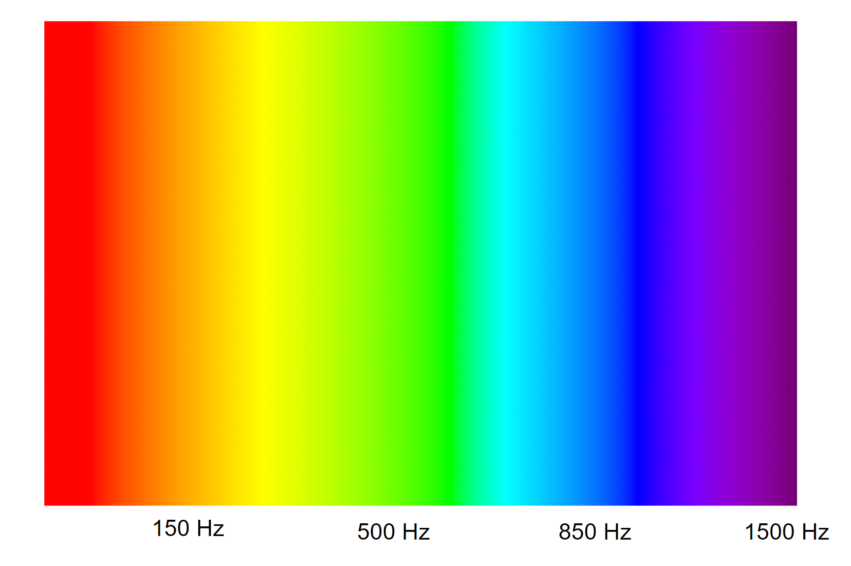
Overall, the results of the disco mode of the lightsaber met all expectations. As mentioned in earlier sections, the frequency of the surrounding sound controls the base color of the lightsaber. As a result, this would mean that each frequency represents a different color. To test this, we conducted a frequency sweep test and the results are summarized in the following image:

Figure 10. Frequency to color in the disco mode

We weren’t able to conduct tests below 150 Hz as this frequency was too low. However, as seen by the figure above, the frequency sweep perfectly corresponds to the RGB color spectrum, where lower frequencies around 150 Hz correspond to orange/yellow, 500 Hz corresponds to green, 850 Hz corresponds to blue, and 1500 Hz corresponds to purple.

Limiting the frequency range to 0 to 1,500 Hz was a design decision. We did this because if the frequency range was too large, then the color changes across the frequency range would become less noticeable; with a smaller range of common frequencies, the color changes are a lot more noticeable. Additionally, the lightsaber, on average, reacts to outside frequency in about 0.2 seconds, which is also something we are very happy with.

Vowel Recognition Results

After getting the cepstral analysis to work, we decided to calibrate the formant frequencies of EE and AH sounds to our voices and see if they match the frequencies from the source Appendix B, 12. The graphs and tables below illustrate the formant frequency 1 and 2 for EE and AH sounds for Berk and Justin:

Table of Collected Formant Frequencies for the AH Sound Made by Justin and Berk

Table of Collected Formant Frequencies for the EE Sound Made by Justin and Berk

Figure 11. Measured first and second formant frequencies for the AH sound

Figure 12. Measured first and second formant frequencies for the EE sound

There are a few important takeaways from these figures. First, the first formant frequencies are a lot more consistent than the second one. This is because our algorithm uses the first instance of peaks that are above the noise threshold, which means it is harder to get the peaks that correspond to higher frequencies, such as the second formant frequencies. This is the reason why we didn’t include the third formant frequency in our analysis and classification because it was too inconsistent to find a pattern in. In this design, the noise threshold was set as 70% of the max intensity, as this was also the value in Bruce Land’s code and it gave promising results that showcased a pattern.

Secondly, the formant frequencies are slightly different depending on Berk or Justin making the vowel sound, which confirms that the expected formant frequencies will be different depending on who is speaking into the microphone.

Finally, using this collected data, we can come up with our own table of formant frequencies of the EE and AH sounds, which were picked by collecting frequencies for each sound across many trials and keeping the mode as the formant frequency.

Table of Formant Frequencies for EE and AH Sounds (Based on Our Results)

After finding the calibrated frequencies for our voices, we adjusted the expected frequencies based on the table above, and ran 20 trials to see the accuracy of the lightsaber. Here are the results for the AH and EE sounds:

Accuracy of EE and AH detection

This result was expected as the first formant frequency of the EE sound is a lot more consistent than that of the AH sound. Overall, we were very happy with this result, which showed a clear pattern that the cepstral analysis was working, and there was indeed vowel detection implemented in our system.

Improvements

Overall, we are extremely pleased with our progress on this project given the time frame was only 5 weeks. However, given more time, we would like to spend more time on the vowel detection mode to increase the accuracy up to 95%. As mentioned in the above section, we weren’t able to detect the third formant frequency properly. If given more time, we would like to try this process with a better microphone, create a more visual debugging method such as using a spectrogram, and spend more time adjusting the noise threshold to find the optimal value.

Safety

There are two safety concerns we thought of while creating our project. Firstly, a lightsaber can be viewed as a weapon, so ensuring that we had a mechanical system that could not be used to hurt anyone. This meant the blade was not sharp or heavy so that if someone was to use it and they struck someone, the person would not be injured.

Secondly, from an audio perspective, we limited the frequency range to 1,500 Hz for the disco mode and 4,000 Hz for the vowel recognition mode. We wanted to restrict the range to incentivize users not to use crazy high frequencies that could cause harm. We only use max intensities for disco mode to encourage the user to not blast extremely intense noise which could damage their ears.

Usability

The usability of the lightsaber has 2 main challenges. The first challenge is due to mechanical design. We weren’t able to find a room to put the battery pack and the mode switching button. As a result, although one can easily lift up this lightsaber, it requires holding the battery pack, which is not the most comfortable experience.

Additionally, the vowel detection mode of the saber is calibrated for Justin and Berk’s voices; thus, the lightsaber doesn’t work as well when other people try to make the EE and AH sound.

Conclusion

We set out to create a lightsaber that would change based on audio input from the outside world and we believed we accomplished our goal. Our disco mode worked seamlessly and created some really interesting color displays. The vowel mode was extremely difficult and does not have perfect accuracy, but shows consistency and that was seen as a big win for us.

There are still several changes we would make given more time. Firstly, we would like to work on the mechanical design in two ways. Increasing the size to fit everything on the inside of the saber excluding the microphone. Secondly, the lightsaber is button activated, and we would utilize the current electrical system instead of our small external button to implement into our system. Thirdly, we would use a stronger microphone to get more consistent audio input to improve our vowel recognition program.

Finally, in terms of usage rights, our design uses the lightsaber from the Star Wars Store  (Appendix B, 14) as the base design and uses code from Bruce Land’s vowel detection experiment (Appendix B, 7 & 8) as well as Hunter Adam’s demo code (Appendix B, 15). Other than these, the entirety of the design and software is created by us. Overall we had a lot of fun building this cool lightsaber, and we are very happy with the final results!

Appendix A (Permissions)

1. The group approves this report for inclusion on the course website
2. The group approves this report for inclusion on the course youtube channel

Appendix B (References Used and Sources)

1. Pi Pico datasheet
2. RP2040 datasheet
3. Digital lowpass filters
4. Fast Fourier Transforms
5. WS2812B datasheet
6. Max 4466 Microphone datasheet
7. Bruce Land HSV2RGB
8. Bruce Land Vowel Detection
9. HSV Illustration
10. HSV to RGB Conversion Image
11. Table of Formant Frequencies of Several Vowels
12. Formant Frequencies of EE and AH
13. Ws2812 PIO Example from pico-examples
14. Lightsaber Used
15. FFT Demo Code

Appendix C (Work Distribution)

Throughout the entire project Berk and Justin worked together at all times on the project. This means we went to the lab together every time we worked on the project and wrote the report together. There was no real work separation as this was a full team effort on all aspects of the project.

Appendix D (Code)

All code files can be viewed in this GitHub repository.